01 Coulomb’s Law (2)

Aim¶

To show the inverse square distance dependence of the electrostatic force between point charges.

Subjects¶

• 5A20 (Coulomb’s Law)

Diagram¶

Equipment¶

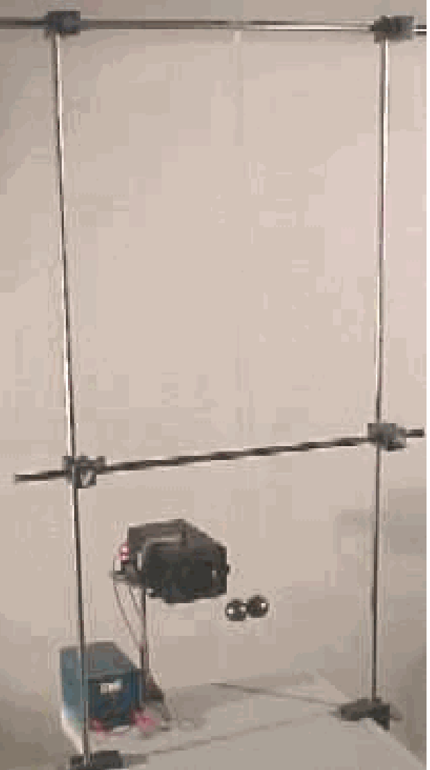
• 2 Graphite-coated ping-pong balls, hanging from a pair of one meter long threads.

• Support (see Diagram).

• Glass rod (see Diagram).

• Red tape, to shift the thread length from $L$ to $0,5 \mathrm{~L}$ (see Diagram PresentationXX).

• Van de Graaff generator.

• Lamp, for shadow projection.

• Overhead sheet with the $\left(n-\frac{r_{1}}{r_{2}}\right.$ ) table (see Explanation).

Presentation¶

The balls are hanging and touch each other. The shadow of the ping-pong balls is projected on the blackboard.

By means of the Van de Graaff generator the two balls are charged and immediately they separate by electrostatic repulsion. While the shadows of the two balls are dancing around towards their equilibrium, the method of the demonstration is explained to the students and to them it is shown that when we suppose the power in Coulomb’s law (1785) is really -2 , the determined distance-ratio should be $2^{1 / 3}=1.259$ (see Explanation). When the two balls have come to rest, the centres of the shadows of the balls are chalk-marked on the blackboard.

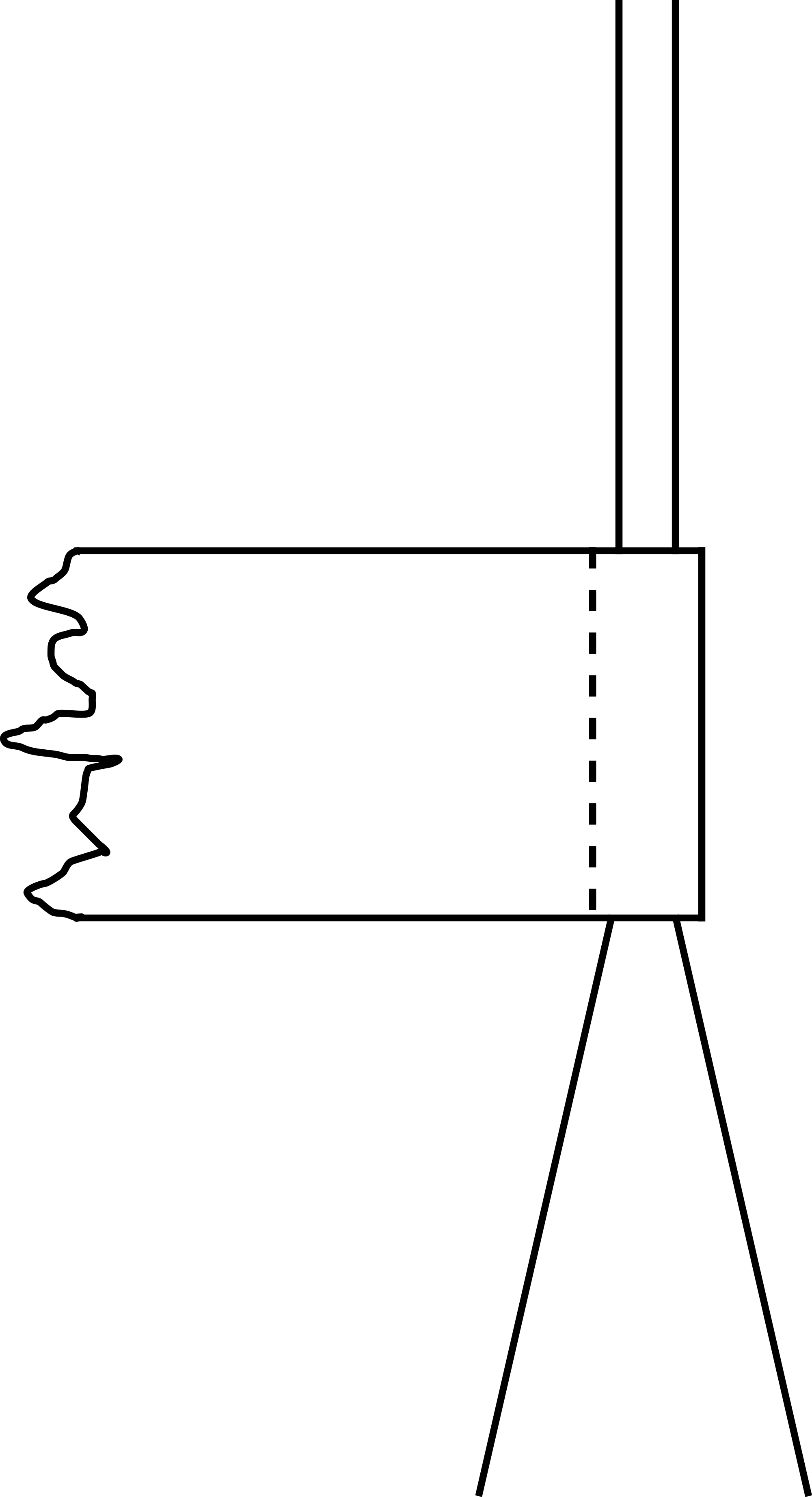
Now the two threads are sandwiched at the halfway point by means of a sliding piece of tape. (This tape is fixed to the threads already before you start the experiment; see Figure 2.)

Clearly can be seen that the two shadows are closer to each other now. Again the centres of the ball-shadows are chalk-marked.

On the blackboard the two separations are measured. (In a trial, we measured 78and $62 \mathrm{~cm}$ respectively.) The ratio is calculated ( $78 / 62=1.258$ ). This value is very close to the value 1.259 mentioned before and so the power in Coulomb’s law being- 2 is supported by this demonstration.

This demonstration gives the opportunity to stress to the students that Coulomb’s law is empirical and in that way very fundamental to the theory of electromagnetism.

That’s why it is very fundamental that measurements around Coulomb’s law are still performed, trying to determine $n$ with increasing accuracy (nowadays -1971- it stands to be accurate to 1 part in 10¹⁶; between 1,99999999999999994 and 2,00000000000000058 )

Explanation¶

Figure 3 shows that in the equilibrium position: $F_{\text {coulomb }}=m g \tan \varphi$.

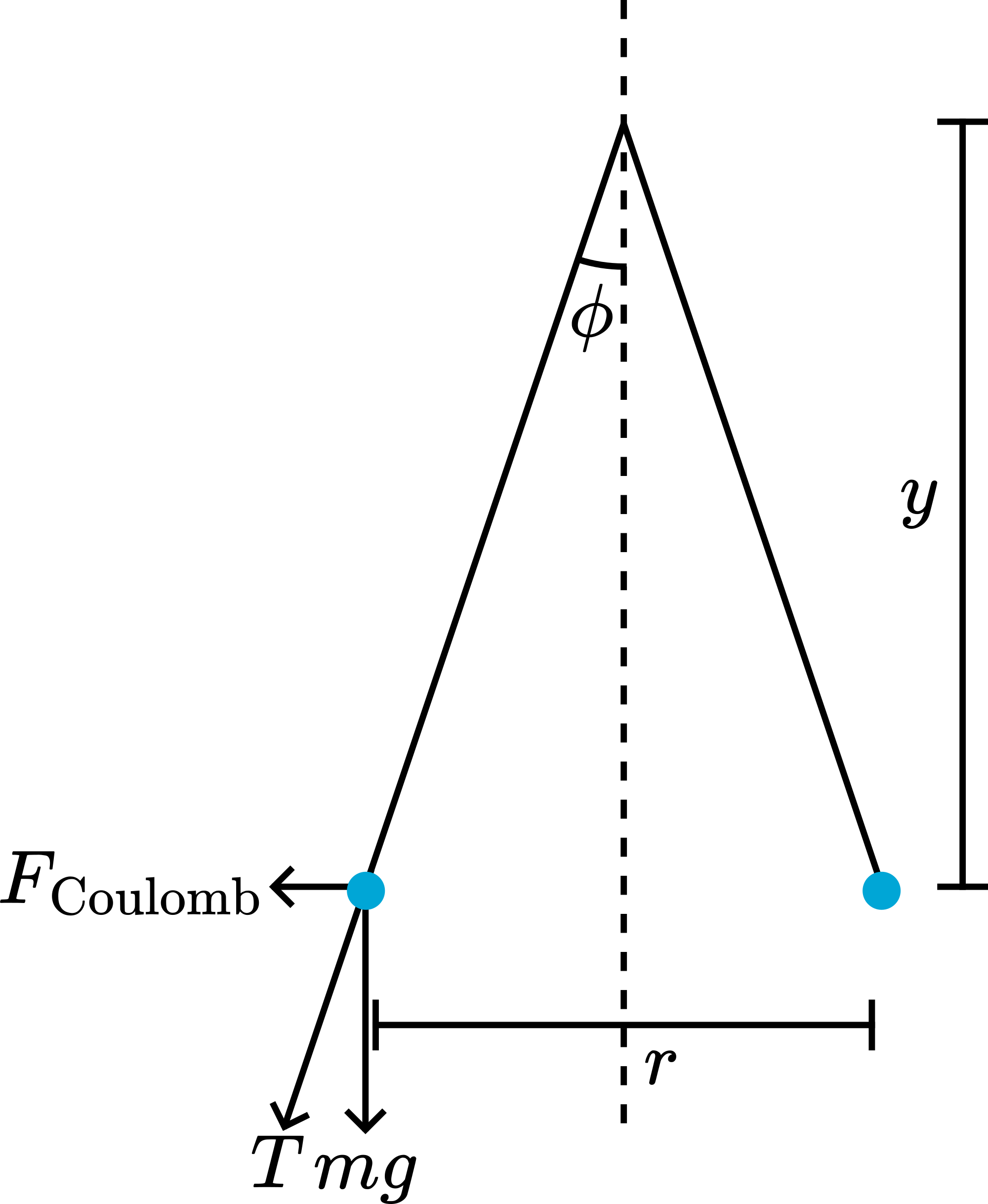
Since $\tan \varphi=r / 2 y, F_{\text {Coulomb }}=\frac{m g r}{2 y}$

Supposing $F_{\text {Coulomb }}=k \frac{q^{2}}{r^{n}}$, our equilibrium equation is $\frac{k q^{2}}{r^{n}}=\frac{m g r}{2 y}$.

$k, q, m$, and $g$ are constants, so $\frac{r^{n+1}}{y}$ has a constant value $\left(\frac{r^{n+1}}{y}=\frac{2 y k q^{2}}{m g}\right.$ )

The first measurement gives us $\frac{r_{1}^{n+1}}{y_{1}}$, the second $\frac{r_{2}^{n+1}}{y_{2}}$. So, $\frac{r_{1}^{n+1}}{y_{1}}=\frac{r_{2}^{n+1}}{y_{2}}$.

Since in our demonstration $y_{1}=2 y_{2}$, we find $\frac{r_{1}^{n+1}}{r_{2}^{n+1}}=\frac{y_{1}}{y_{2}}=2$, and so: $\frac{r_{1}}{r_{2}}=2^{\frac{1}{n+1}}$

For different values of $n$ we calculate for $\frac{r_{1}}{r_{2}}$ :

In this way measuring $r_{1}$ and $r_{2}$ will give us the value for $n$.

The mentioned measurement in the Presentation with $r_{1}=78 \mathrm{~cm}$ and $r_{2}=62 \mathrm{~cm}$ presents the ratio $\frac{r_{1}}{r_{2}}=1,258$.. the table above shows that this produces a value for $n$ very close to 2 .

Remarks¶

• Measuring $r_1$ and $r_2$ must be done with some care. For instance when you measure $r_2$ being $63\mathrm{~cm}$ instead of $62\mathrm{~cm}$ you find $n=2.2(5)$ instead of $n=2.0(2)$.

• When charge leaks away during the demonstration the measured $r_2$ will be too low making $\frac{r_1}{r_2}$ higher and $n$ will appear as a higher value. (So usually this will happen.)

• At $3/4$ from the upper side of the support a horizontal bar is placed (see Diagram). This makes that when the balls move when they deflect, they remain in the same vertical plane. Without this bar the balls will start to rotate, making a useful shadow projection impossible. Nowadays we use a thin double thread instead of a metal bar; a metal bar that close to the balls disturbs the E-field more than a thin thread. The balls hang between the double, horizontal threads.

Sources¶

• Ehrlich, R., Why Toast Lands Jelly-Side Down: Zen and the Art of Physics Demonstrations, pag. 146-147

• Mansfield, M and O’Sullivan, C., Understanding physics, pag. 443 and 467

• Young, H.D. and Freeman, R.A., University Physics, pag. 674-679

• Buijze W. en Roest R., Inleiding electriciteit en Magnetisme, pag. 11, eerste zin.

• Giancoli, D.G., Physics for scientists and engineers with modern physics, pag. 549-551 and 586!

Supplement¶

Historical results

• Henry Cavendish (1770):
  $\quad\quad|\varepsilon|\leq 0.02$

• James Clark Maxwell(1879):
  $\quad\quad|\varepsilon|\leq 5\cdot 10^{-5}$

• E.R. Williams, J.E. Faller and H.A. Hill (1971):
  $\quad\quad|\varepsilon|\leq (2.7\pm 3.1)\cdot 10^{-16}$