D30 Rain of balls

Aim¶

To show by means of a large scale model the results of the interaction between gasmolecules and a wall.

Subjects¶

• 4D30 (Kinetic Motion)

Diagram¶

Equipment¶

• 50 ping-pong balls.

• Pipe, $l=2 \mathrm{~m}$; internal diameter $40 \mathrm{~mm}$, with a pin through its end.

• Large container to catch the rain of ping-pong balls.

• Force sensor.

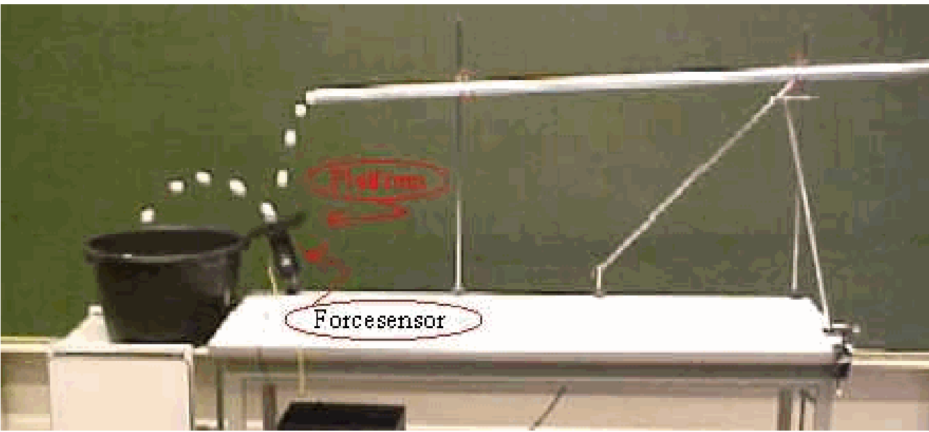
• Platform. This is an acrylic sheet, $22\times22\times.2\mathrm{~cm}$, mounted to the forcesensor.

• Data-acquisition system with interface.

• Projector to project an image of the monitorscreen.

Presentation¶

Preparation.¶

The pipe is filled with ping-pong balls and clamped slightly slanting just to enable the balls to roll by themselves. The force-sensor with the acrylic platform is fixed to the table and stands oblique, that much that when a ping-pong ball falls on it, this ball jumps into the large container (see Diagram). The software of the data-acquisition system displays the force on the platform in a time-graph and average force on a digital display. Use the tare-button on the force-sensor to “zero” it.

Presentation¶

First drop, by hand, one ball on the platform and monitor the force-time graph. Use this graph to explain to your students how the demonstration set-up functions and what the readings of the graph and meter tell us.

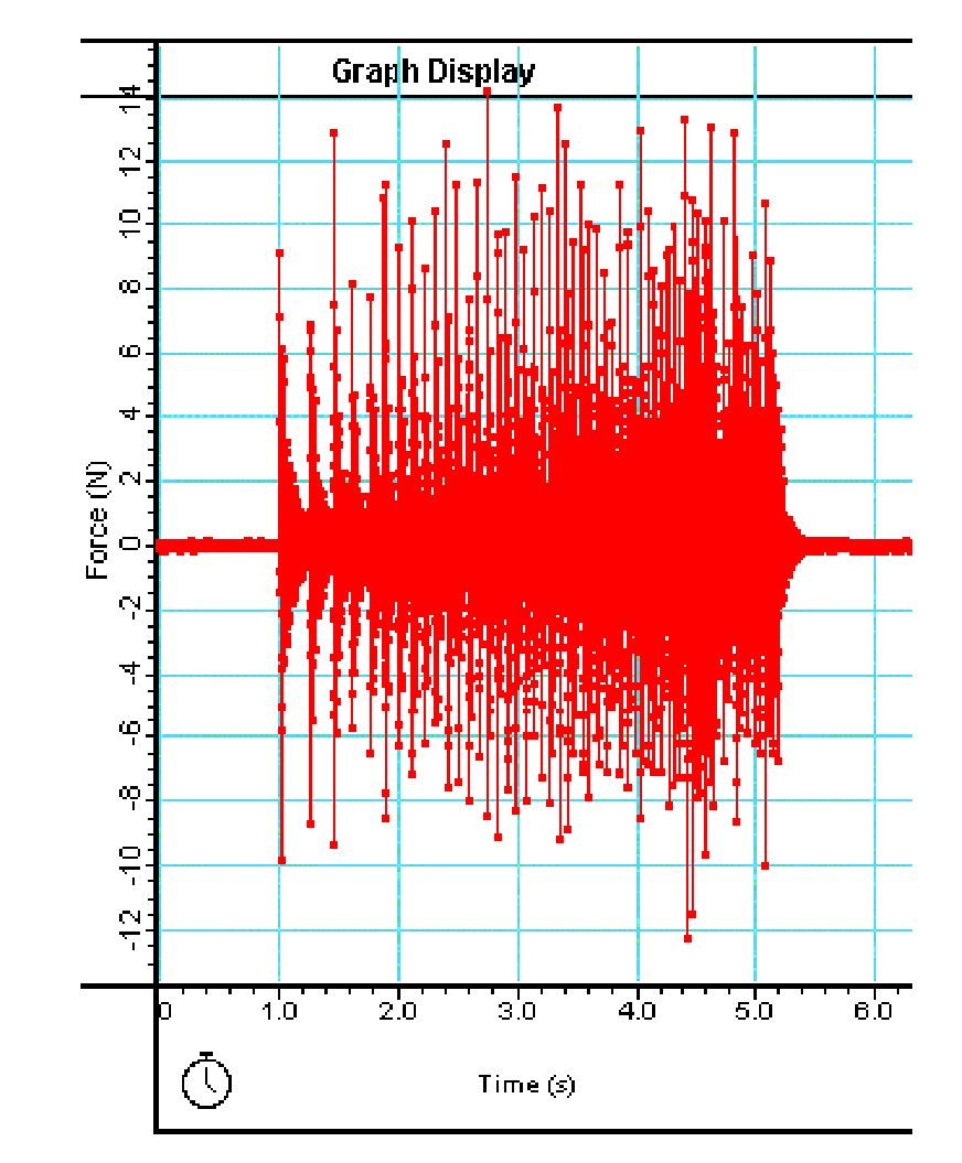
• The force diagram shows a strong oscillation of the platform. Using the zoom function of the software, it can be shown that at the beginning there is a strong positive impulse: $F$ - $\Delta t$-area. (The subsequent oscillation averages to zero.)

Reset the software to a recording mode and then pull the pin out of the end of the pipe: A train of balls falls onto the platform. All students’ attention might be attracted to the falling balls, so draw their attention also to the ongoing registration of the graph and digital meter. After the rain of balls is over, the results can be discussed. Especially worthwhile are the high force readings of the individual balls (up to $14 \mathrm{~N}$! See Figure 2) in contrast to the low average force on the digital scale $(0.08 \mathrm{~N})$.

Explanation¶

The force exerted by an individual ping-pong ball equals $\vec{F}=\frac{\Delta \vec{p}}{\Delta t}$. F can be that high since $\Delta t$ (the time the ball touches the platform) is very small. The kinetic theory of gasses shows that the force on the wall of a container filled with a gas is proportional to the average scalar product of momentum and velocity of the gas molecules $F=\frac{1}{3} \frac{N A}{V}(\vec{p} \cdot \vec{v})$.This demonstration shows the proportionality with $\vec{p}$.

Force due to one collision¶

When we examine the force-time graph it can be seen that the rise time of $\mathrm{F}$ during the collision is in the order of $1 \mathrm{msec}$ (see the registration in Figure 3).

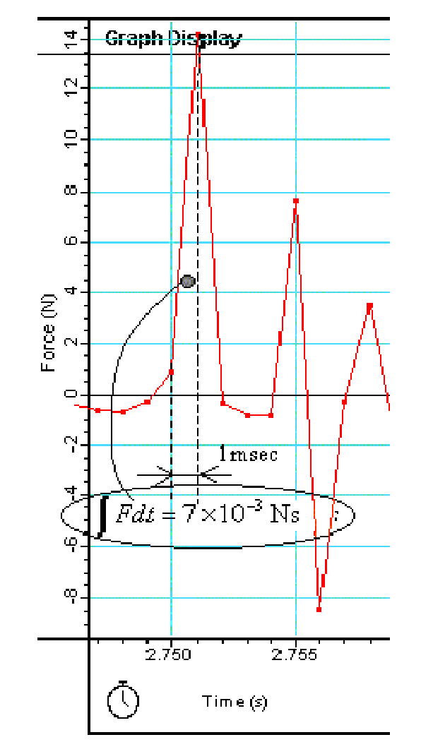
The ping-pong ball has a mass of $2.5 \times 10^{-3} \mathrm{~kg}$ and falls a height of around $0.5 \mathrm{~m}$, so at the collision with the platform it has a speed of around $3 \mathrm{~m} / \mathrm{s}$. So, the momentum at collision is $7.5 \times 10^{-3} \mathrm{kgm} / \mathrm{s}$. The impulse $\int F d t=\Delta p$. So, in this case $\int F d t$ should read $15 \times 10^{3}$ Ns. Using the function “integrate” of the software over the corresponding impulse-area will produce that result. Since the collision is not perpendicular and not completely elastic, the registered $\int F d t$ will be lower than $15 \times 10^{-3} \mathrm{Ns}$.

Average force¶

In our macroscopic world we experience the average force. After a collision with a pingpong ball the platform shows a damped free oscillation. Such a free oscillation averages to $\mathrm{F}=0$. The force-time graph shows $5015 \times 10^{-3}$-collisions in about 4 seconds time average to around $0.19 \mathrm{~N}$. Selecting the area between of 4 seconds the software shows this as the mean $y$-value.

Remarks¶

• The platform that is hit by the ping-pong balls is not an ideal rigid wall as meant when you treat the details of the kinetic theory of gasses. As the registered graph shows, the platform vibrates strongly (in many modes) after a hit. However, when we average the registered forces of these vibrations (so average the whole registered graph of a hit except the “real hit” at the beginning) we find ‘zero’ as a result.

Sources¶

• Mansfield, M and O’Sullivan, C., Understanding physics, pag. 247-250

• PASCO scientific, Instruction Manual and Experiment Guide, pag. CI-6537