01 Magnetic Fields

Aim¶

To show the distance-dependence of magnetic fields in three situations: of a straight wire carrying a current; of a “monopole” and of a dipole.

Subjects¶

• 5H10 (Magnetic Fields)

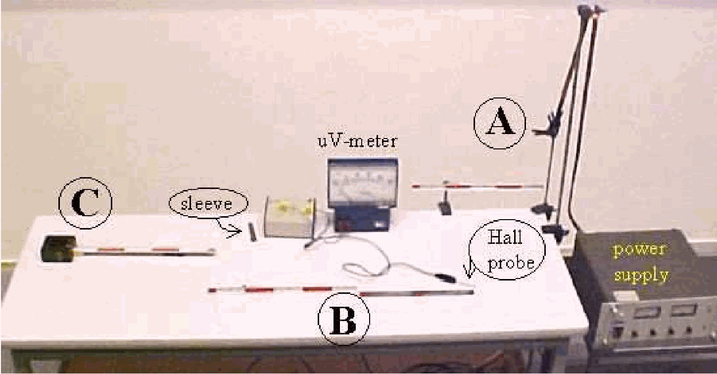
Diagram¶

Equipment¶

• Brass rod, diameter $8 \mathrm{~mm}$.

• Power supply, $100\mathrm{~A}$ DC.

• Thick leads to conduct $100 \mathrm{~A}$.

• Two bar magnets.

• Horseshoe magnet.

• Hall probe (tangential).

• Hall-probe power supply.

• Sleeve of metal to zero the Hall probe.

• UV-meter.

• Three short rulers, $30 \mathrm{~cm}$.

Presentation¶

A Hall probe is used to measure the B-field. The reading is in $u \mathrm{~V}$ (indicating the Hall-emf). In the demonstration we use the $0-10$ scale of the $U V$-meter in $0-10$ arbitrary B-field units.

Presentation A (see Diagram A)¶

In the brass rod a current of $100 \mathrm{~A}$ is flowing, supplied by the power supply. The Hall probe measures the $B$-field at $1 \mathrm{~cm}$ distance from the center of the brass rod. The measurement is done again at $2 -$ and $4 \mathrm{~cm}$. We measure respectively 4,2 and 1 unit of magnetic field. This shows clearly the $R^{1}$ dependence of the magnetic field in this situation.

Presentation B (see Diagram B)¶

We create a monopole by placing two long magnets head to tail. In that way, the North- and South pole are far away from each other. So, in the neighborhood of the North pole the influence of the South pole can be neglected.

First we need to detect where this monopole is situated. The magnet bar is placed on an overhead projector and covered with a plexiglass sheet. Scattering iron filings on the sheet will show the shape of the magnetic field by the orientation of the filings. It is observed that the field lines “originate” from a point about $1 \mathrm{~cm}$ inside the bar magnet (see Figure 2).

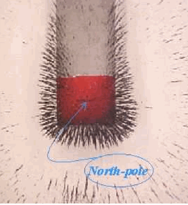
Then the magnetic field is measured. The Hall probe is shifted towards the monopole until a deflection of 8 units. The distance away from the monopole is read on the ruler. Then the distance is doubled, and the meter indicates: 2 units. These two measurements illustrate the $R^{2}$ dependence of the magnetic field in this situation.

Presentation C (see Diagram C)¶

As a dipole we use a strong horseshoe magnet. First we indicate from where we measure the distances and which orientation we will use (see Figure 3). We start perpendicular to the magnet. The probe is shifted until we measure 8 units on the meter. The distance from the dipole is measured on the ruler. Then we ask the students what will be read from the meter when the distance is doubled.

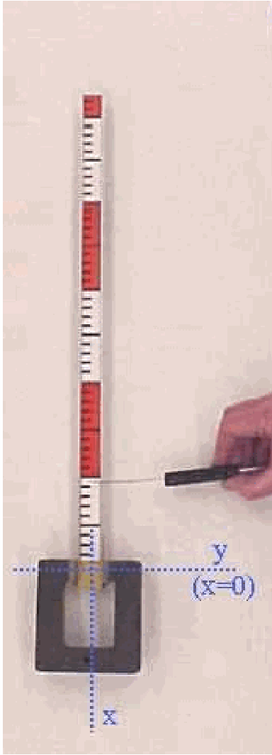
When we measure we come to 1 unit, illustrating the $R^{-3}$ dependence of the $B$-field in case of a dipole.

The same procedure is followed when $R$ is in the direction of the dipole (this is along the $y$-axis, see Figure 3). The same dependence will be found.

Also any other orientation can be measured with the same result.

Explanation¶

Textbooks explain the three situations presented.

Presentation A¶

In this presentation applying the Biot-Savart law gives the field near a long straight wire: $B=\frac{\mu_{0} I}{2 \pi R}=2.10^{-7} \frac{I}{R}$. The factor 10^-7 explains why such a high current is needed in this presentation (for $I=100 \mathrm{~A}$ and $R=1 \mathrm{~cm}$, we find $B=2 \mathrm{mT}$ ).

Presentation B¶

For a magnetic monopole $B=\frac{\Phi_{m}}{4 \pi R^{2}}, \Phi_{\mathrm{m}}$ is the total magnetic flux from the pole.

Presentation C¶

For a magnetic dipole: $B=\frac{\mu}{2 \pi} \frac{\vec{m}}{R^{3}}, m$ being the magnetic dipole moment.

Remarks¶

• In all three demonstrations more points can be measured, but since it is “only” a demonstration a limited amount of situations suffices to stress your point.

• In the explanation the R-dependence of the magnetic field can also intuitively be compared to the already known situation of the E-field of a point-charge (presentation B) and the E-field of a dipole (presentation C).

Sources¶

• Buijze W. en Roest R., Inleiding electriciteit en Magnetisme, pag. 109-111

• Giancoli, D.G., Physics for scientists and engineers with modern physics, pag. 719-720

• Mansfield, M and O’Sullivan, C., Understanding physics, pag. 484-485