01 Electromagnetic Waves (Lecher Lines)

Aim¶

To show wave characteristics of electromagnetic waves (UHF) on conducting bars (Lecher lines), in air and in water.

Subjects¶

• 5N10 (Transmission Lines and Antennas)

Diagram¶

Equipment¶

• UHF-transmitter.

• Dipole loop.

• Transmitter dipole model (box with rope, $\mid=\lambda$; see Figure1E).

• Lecher system, a set of metal rods and loops of different length:

  • 4 rods of $3 \lambda / 4$

  • 1 rod, $\lambda / 4$

  • 1 loop, $\lambda / 2$ ( $35 \mathrm{~cm}$ )

  • 1 loop, $\lambda / 4$

  • 1 shorting plug.

  • 3 PVC rods to support conducting rods.

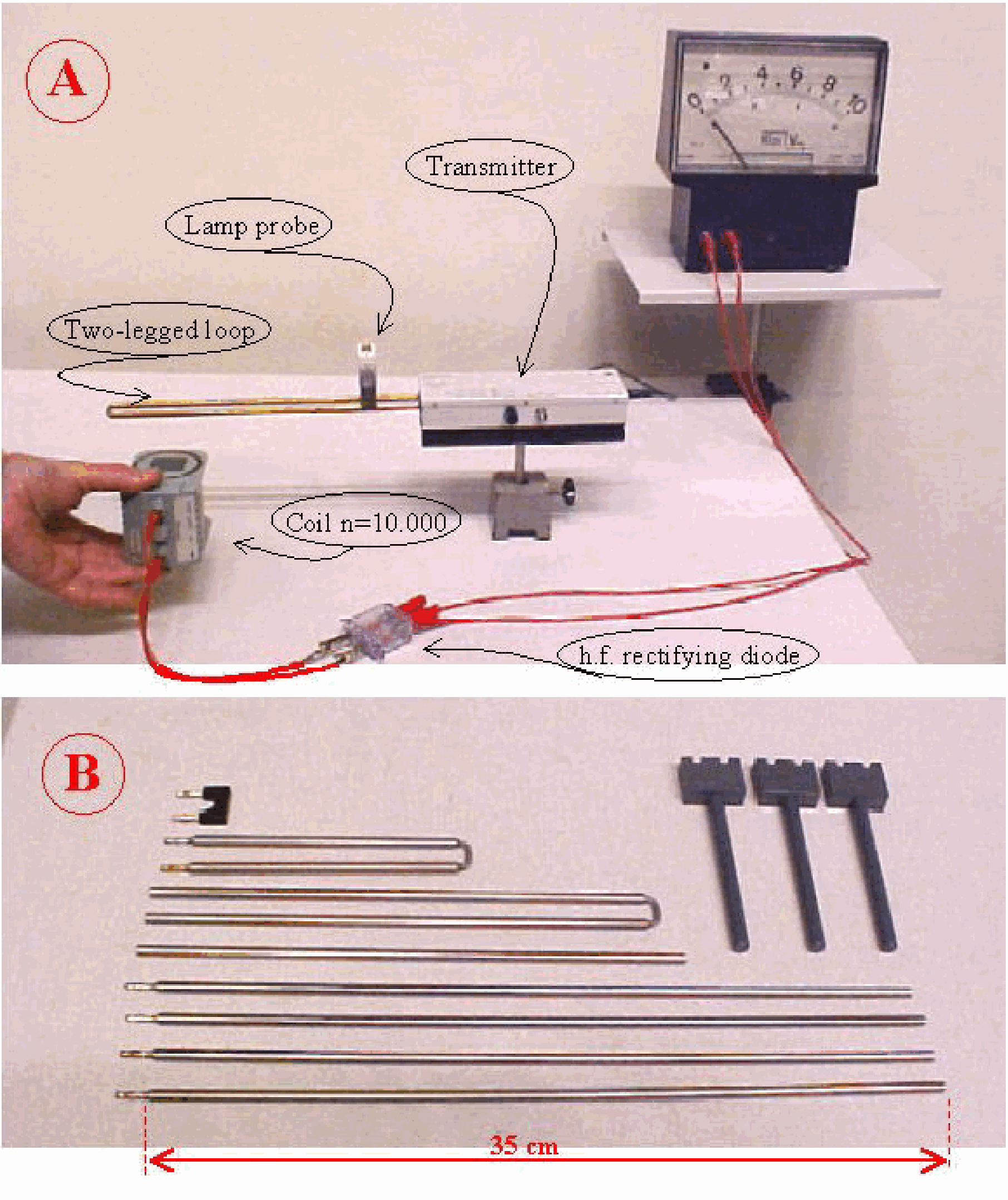
• Lamp-probe for E-field. This is a lamp socket with lamp, $3.8 \mathrm{~V} / 70 \mathrm{~mA}$, fitted in a PVC block in such a way that the leads of the socket are inside the plastic block and cannot be touched.

• Receiver dipole with lamp $3.8\mathrm{~V}/70\mathrm{~mA}$.

• Coil, $n=10.000(R=1350 \Omega)$.

• Receiver dipole with h.f. rectifying diode.

• $100 \mathrm{vA}(1 \mathrm{k} \Omega$ ) demonstration meter.

• Aluminum sheet.

• Metal grated sheet

• Water tank with long and short $\lambda / 2$ dipole with lamps $3.8 \mathrm{~V} / 70 \mathrm{~mA}$.

• Demineralized water.

• Ohp-sheet with Figure 3.

Safety¶

• No remarks. Electromagnetic waves

Presentation¶

Preliminary explanation.¶

The UHF transmitter box contains a circuit that resonates at around $434 \mathrm{MHz}$. In the output of this circuit, conducting rods of different length can be plugged in. When the wavelength $(\lambda)$ of the E-field of this $434 \mathrm{MHz}$ signal is calculated, we find $\lambda$ is around $70 \mathrm{~cm}$ (the electric field $E$ travels at $3 \times 10^{8}$ $\mathrm{m} / \mathrm{s}$ ).

A. STANDING ELECTROMAGNETIC WAVES ON CONDUCTORS.¶

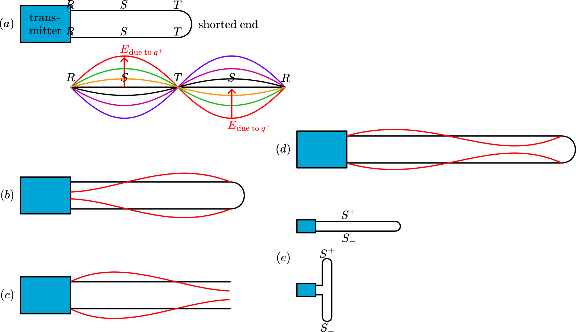
The metal two-legged loop, having a length of $35 \mathrm{~cm}$ (Lecher-line), is plugged into the transmitter output. Place the lamp-probe with its pvc block on the two-legged loop and slide it along the legs of the loop (see Diagram A). The lighting lamp shows: $V_{R-R}=0$, rising to $V_{S-S}=m a x$. and then diminishing to $\mathrm{V}_{\mathrm{T}-\mathrm{T}}=0$.

This pattern can be understood when showing that a full standing E-wave fits into the total length of $70 \mathrm{~cm}$. Then there are E-nodes at $17.5 \mathrm{~cm}(\lambda / 4)$ and at $52.5 \mathrm{~cm}(3 \lambda / 4)$. At $35 \mathrm{~cm}(\lambda / 2)$ there is an antinode. Figure1A shows this E-pattern and clarifies that maximum potential difference occurs between $\mathrm{S}$ and $\mathrm{S}$. (S-S is an in intensity oscillating dipole.)

Then the coil with $n=10.000$ is connected to a $100 \mathrm{vA}$ demonstration meter via the h.f. rectifier diode (see Diagram A). The coil is placed on a cart and slides slowly and close ( $2 \mathrm{~cm}$ distance) along one of the legs of the conducting rods. The demonstration meter shows where induction along the leg happens, it shows the nodes and anti-nodes of the magnetic field $B$ along the conducting rod; so it shows the standing current pattern in the conducting rod. We find B-nodes and anti-nodes on the places opposing those of the E-field. (see also: Remarks)

Then longer two-legged loops are build (Lecher system; see Diagram B). This Lecher system makes i possible to investigate the standing electromagnetic wave in longer variants, either shorted or open ended (Figure 3B, C and D are possible examples). Sliding the lamp-probe and/or the coil in these examples will strengthen the idea of standing E- and B-waves on the conductors.

(When needed to illustrate that a standing wave is related to length, the demonstration “Handheld standing waves” in this database can be used. Also “Kundt’s tube” can be used as an analogy.)

B. ELECTROMAGNETIC WAVES IN AIR (DIPOLE LOOP).¶

The dipole loop is fitted into the transmitter output. This loop has the same total length as the metal two-legged loop of $35 \mathrm{~cm}$ used in the first demonstration. The difference is that this dipole loop is folded in a different way: On the overhead projector the transmitter dipole model with rope is used to demonstrate the similarity between the two-legged $\lambda / 2$-loop and the dipole loop (see Figure1E). This dipole form is such that the dipole moment ( $p$ ) of the oscillating positive and negative charges on the loop is maximum, because $d$ is maximum in $p=q d$ ( $q$ being the charge at $\mathrm{S}$ ). (The resulting $\mathrm{E}$-field is proportional to $p$ and the irradiance proportional to $p^{2}$; so it is profitable to make $p$ as large as possible [see E.Hecht’s “Optics”, pg. 62 or another text on electric dipole radiation]).

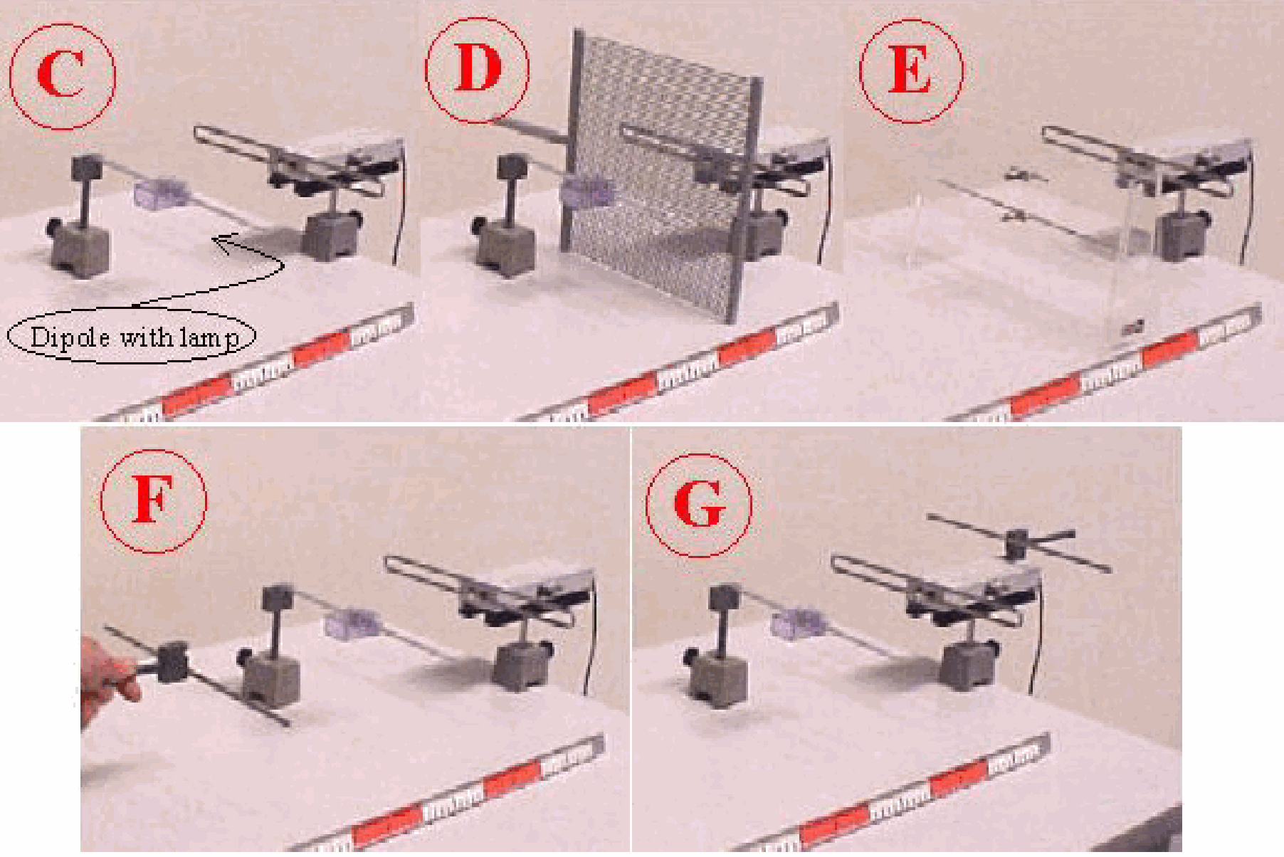
• Radiation. When the transmitter is switched on, the receiver dipole with lamp shows that at a distance there is also an electric filed (see Diagram C). The measured intensity depends on the distance. Conclusion can be that a field is radiated by the dipole loop.

• Absorption. The receiver dipole is stationed horizontally at around $20 \mathrm{~cm}$ distance from the transmitter dipole loop. The absorption of different materials is investigated in placing sheets or blocks of material between the transmitter and receiver dipole. We try: wood, glass, Perspex, Teflon, stone bricks, my arm, water. Only my arm shows absorption, the other materials are transparent to the radiation.

• Polarization. Observing the lamp in the receiver dipole while rotating it shows that the E-field is polarized and stands in the direction of the loop dipole that is plugged into the transmitter. Placing a metal grated fence between the transmitter and the receiver and slowly rotating thi grating, affirms the polarization of the E-field (see Diagram D).

• Reflections. At $17.5 \mathrm{~cm}$ ( $1 / 4 \lambda$ from the transmitter the receiver dipole is placed. At $35 \mathrm{~cm}$ an Al sheet is put in the radiated beam: the receiver dipole shows a rather strong increase in intensity. Shifting the Al sheet produces variations in intensity on the receiver dipole. Putting in at $52.5 \mathrm{~cm}$ shows a reduction of intensity, while putting in at $70 \mathrm{~cm}$ should show again an increase in the intensity; this is faintly visible. Then from $70 \mathrm{~cm}$ the distance is decreased again and after the maximum intensity at $35 \mathrm{~cm}$ we approach the receiver dipole still closer causing finally the lamp to dim completely. This last part of this demonstration shows that there is an anti-node at the reflecting sheet. All this can be explained by standing E-waves, similar as in the demonstrations with the conducting rods. When the sheet is replaced by a metal rod of the same length as the receiver dipole, the same demonstrations as with the metal sheet can be performed, also finally completely dimming the lamp of the receiver dipol (see Diagram F). (Instead of using a metal rod in order to increase the intensity at reflection, you can as well use your arm!)

But now we continue!

Move the metal rod from the receiver dipole towards the transmitter and the lamp of the receiver dipole remains extinguished. While close at the transmitter this can be explained suggesting that the rod, that also receives energy from the transmitter, emits the energy again but now with a phase-change of $\pi$. A simple test then is to touch the metal bar with your hand in order to absorb part of the energy received by the metal bar and while doing so you will see that while touching, the lamp of the receiver dipole lights again. Another test of the $\pi$-phase-shift-hypothesis is placing the metal bar $1 / 4 \lambda$ behind the transmitter dipole in an attempt to increase the lighting of the receiver dipole and amazingly (to the students) this succeeds (see Diagram G). (A/so here you can use your arm as a reflector.)

• EM-waves in water. At $17.5 \mathrm{~cm}$ from the transmitter dipole the acrylic box with two lamps is placed (see Diagram E). The lamp with the longer metal rods will lighten. Then demineralized water is poured into the box. When the water level reaches the longer metal rods, the lamp turns out. When finally the water level reaches the short metal rods the lamp connected to those rods lights up. This shows that the wavelength in water is much shorter than the wavelength in air (the rods are 9 times shorter). This corresponds with the dielectric constant of water being around 80: $c_{\text {medium }}=\frac{C}{\sqrt{\varepsilon_{r} \mu_{r}}} \cdot c_{\text {water }}=\frac{1}{9} c$, making $\lambda 9$ times smaller. Behind the waterbox the wavelength is again $70 \mathrm{~cm}$ as placing of the lamp probe with longer rods at that position will show.

Explanation¶

Figure 3 explains the polarized E-field that is produced by the loop dipole. This loop dipole is effectively the two-legged loop of Figure 3A, but folded in a different way. Figure1E makes clear that there is a resulting E-field pulsating with a frequency of $434 \mathrm{MHz}$. The explanation is already done in the description “PresentationXX”. More details can be found in the presented “SourcesXX”.

Remarks¶

• The $\pi/2$ phase-shift between $E$ and $B$ on the Lecher line should not be confused with the in-phase situation of $E$ and $B$ of the EM-field in vacuum (air). The in-phase situation belongs to the EM-field as detected relatively far away from the emitting dipole.

• Detecting the magnetic field is very difficult, because the $B$-field is very, very weak. It is even advisable not to perform this part of the demonstration with this equipment. A much stronger sender is needed for that!

• Do not touch the metal bar and Al-sheet and the metal grated fence with your hands, because then energy is absorbed and the metal is no perfect reflector any longer.

• Mind that anything made of metal in the neighborhood of your demonstration is a possible reflector. (For instance the metal frame of your table.)

• In the demonstration with the Lecher-lines mind that the detector lamp is not touching the conducting lines, because this will destroy your lamp.

Sources¶

• Buijze W. en Roest R., Inleiding electriciteit en Magnetisme, pag. 172-173.

• Giancoli, D.G., Physics for scientists and engineers with modern physics, pag. 792-794.

• Hecht, Eugene, Optics, pag. 43-46 and 62-63.

• Leybold Didactic GmbH, Gerätekarte, pag. 58751-58755.

• Vogel, H, Physik, pag. 290-299.