9. Measurements and their uncertainty

9.1. Pre/Post-test

This test is for testing your current skills in Python. You can use it in two ways:

• pre-test: to test your skills beforehand. If you are already proficient in Python, and can do this test within approximately 15 minutes, you can scan through the notebook rather than carfefully reading each sentence.

• post-test: test your skills after Notebook 6. Check whether you learned enough.

Diode

In an experiment 10 measurements were taken of the voltage over and current through a Si-diode. The results are displayed in the following table together with their uncertainties:

I (μA)	\(\alpha_I\) (μA)	V (mV)	\(\alpha_V\) (mV)
3034	4	670	4
1494	2	636	4
756.1	0.8	604	4
384.9	0.4	572	4
199.5	0.3	541	4
100.6	0.2	505	4
39.93	0.05	465	3
20.11	0.03	432	3
10.23	0.02	400	3
5.00	0.01	365	3
2.556	0.008	331	3
1.269	0.007	296	2
0.601	0.007	257	2
0.295	0.006	221	2
0.137	0.006	181	2
0.067	0.006	145	2

The diode is expected to behave according to the following relation: \(I = a(e^{bV}-1)\), where \(a\) and \(b\) are unknown constants .

Exercise: Use the curve_fit function to determine whether this is a valid model to describe the dataset. Is the found parameter \(a\) in agreement with the value found in another experiment \(a_{2} = 2.0 \pm 0.5\) nA?

Hint: use a logscale on the y-axis

I = np.array([3034,1494,756.1,384.9,199.5,100.6,39.93,20.11,10.23,5.00,2.556,1.269,0.601,0.295,0.137,0.067])*1e-6
a_I = np.array([4,2,0.8,0.4,0.3,0.2,0.05,0.03,0.02,0.01,0.008,0.007,0.007,0.006,0.006,0.006])*1e-6
V = np.array([670,636,604,572,541,505,465,432,400,365,331,296,257,221,181,145])*1e-3
a_V = np.array([4,4,4,4,4,4,3,3,3,3,3,2,2,2,2,2])*1e-3

---------------------------------------------------------------------------
NameError                                 Traceback (most recent call last)
Cell In[1], line 1
----> 1 I = np.array([3034,1494,756.1,384.9,199.5,100.6,39.93,20.11,10.23,5.00,2.556,1.269,0.601,0.295,0.137,0.067])*1e-6
      2 a_I = np.array([4,2,0.8,0.4,0.3,0.2,0.05,0.03,0.02,0.01,0.008,0.007,0.007,0.006,0.006,0.006])*1e-6
      3 V = np.array([670,636,604,572,541,505,465,432,400,365,331,296,257,221,181,145])*1e-3

NameError: name 'np' is not defined

9.2. Learning objectives

Now that we know how to do some basic Python, it is time to use it to understand features and the nature of physical measurements.

In this notebook, we will introduce you to measurements, variance in repeated measurements, and measurement uncertainties. If we do calculations with a value with an uncertainty, we end up with an answer that has an uncertainty as well… But how do we calculate this uncertainty? Moreover, we often do not calculate a value on a single set of repeated measurements but rather on datasets with various mean values of repeated measurements. How do we properly analyse these data? For each topic, a summary is given. What is new, compared to the previous notebooks, is that we have * assignments. These are not mandatory, but can be made to help you improve your knowledge of Python and data-analysis.

Now that we know how to do some basic Python, it is time to use it to understand features of physical measurements. It is very useful to study the chapter in the online manual as well!

After completing this notebook, you are able to:

• calculate the mean, standard deviation and uncertainty of a dataset

• report findings using the scientific conventions

• understand and use Gaussian and Poisson distribution

• identify outliers

• carry out an agreement analysis

• calculate how uncertainties propagate when calculations are performed

9.3. Introduction

In natuurkundige experimenten probeer je verbanden of bepaalde waarden zo goed mogelijk vast te leggen. Wat zo goed mogelijk dan precies inhoudt, blijft nu nog even onduidelijk. Wat hopelijk wel meteen duidelijk is, is dat we die waarden vrijwel nooit direct vast kunnen stellen. We voeren verschillende experimenten uit om data te verzamelen waarmee we het verband kunnen bepalen en vervolgens zo goed mogelijk de verschillende parameters in dat verband vast te stellen.

Het lukt echter nooit om de exacte waarde(n) van die parameter(s) vast te stellen: bij elke nieuwe meting zullen er kleine fluctuaties zijn (zeker als je heel precies meet). In de loop der tijd hebben we onze experimenten kunnen verbeteren, en kunnen we in kortere tijd meer metingen doen. Dit zorgt er dan ook voor dat in de loop van de geschiedenis constanten, zoals de constante van Planck, steeds beter bepaald zijn en dat de waarde in de loop der jaren verschilt.

Het gevolg van het nooit precies kunnen vast stellen van een waarde is dat als je gaat werken met die waarde je eindantwoord ook nooit perfect (gedetermineerd) is. Er zal altijd een onzekerheid zijn wat de precieze waarde daadwerkelijk is. In dit hoofdstuk leer je hoe de onzekerheid in een gemeten waarde doorwerkt in het eindantwoord (de basis, significante cijfers en bijbehorende rekenregels, ken je al), en hoe je die onzekerheid zo klein mogelijk maakt.

Note

De woorden meetfout en meetonzekerheid lopen vaak door elkaar heen. In veel gevallen zou meetonzekerheid preciezer beschrijven wat er bedoeld wordt. Een meetfout impliceert dat je iets echt fout doet, zonder dat je daar iets aan kunt doen. De fout komt inherent voort uit het gebruik van een instrument, van het meten zelf. In dat geval zou het dus netter zijn om te praten over de onzekerheid. Alhoewel we hier heel zorgvuldig proberen het onderscheid te maken, gebeurt het in het algemeen taalgebruik dat de twee termen onbedoeld verwisseld worden.

9.4. Goal

Een volledige data-analyse zal vaak bestaan uit de volgende drie fasen:

1. het bepalen van de betrouwbaarheid van individuele metingen en de dataset als een geheel;

2. het vinden en bepalen van het patroon in de data met daarbij de bepaling van de variabelen met hun bijbehorende onzekerheden;

3. een optimale data(re)presentatie om te overtuigen van fasen 1 & 2.

Het doel van dit onderdeel van het natuurkundig practicum is elk het ontwikkelen van een dieper begrip van de bovenstaande fasen en het leren toepassen van de bijbehorende technieken.

9.5. Quantities, units, dimension-analysis and constants

In de natuurkunde meten we fysische grootheden. We onderscheiden vectoren (grootheden met een richting \(\vec{F}\) (N)) en scalairen (grootheden met alleen een waarde (\(m\) (kg)). De grootheid wordt schuingedrukt (\(U\)), bijbehorende eenheid rechtop (V).

Er zijn vijf veel gebruikte standaardeenheden (kg, m, s, K, C). Er is ook nog een zesde standaardeenheid die je minder vaak tegen komt (cd). Alle andere eenheden zijn afgeleid van deze standaardeenheden. De afleiding van de eenheid gebeurt op basis van de formule:

Voorbeeld: Afleiding van J/s

\(P = F\cdot v\)
[J/s] = [kg m s\(^{-2}\)] \(\cdot\) [m s\(^{-1}\)] = [kg m\(^{2}\) s\(^{-3}\)]

Op een zelfde wijze, op basis van eenheden (dimensie-analyse), kun je formules afleiden als je weet welke grootheden mogelijk een rol spelen. Bij het tweedejaarsvak Fysische Transportverschijnselen zal daar veel dieper op ingegaan worden. Wil je weten hoe je een dimensie-analyse uitvoert? Kijk dan eens dit filmpje:

Bij veel experimenten waarin je een verband bepaalt, maak je gebruik van een constante, bijvoorbeeld de constante van Planck. CODATA heeft een mooi lijstje gemaakt van die constanten met hun bijbehorende (relatieve) onzekerheid. Maak gebruik van deze referentie bij het opzoeken en gebruik van natuurkundige constanten.

Exercise 9.1

Gegeven de vergelijking \(F=k \cdot v^2\), wat is de eenheid van \(k\) uitgedrukt in de SI-eenheden (kg,m,s,C,K)?

Solution to Exercise 9.1

\(F = k \cdot v^2 \)

\([kg \frac{m}{s^2}] = [..] \cdot [\frac{m^2}{s^2}]\)

\(k → [\frac{kg}{m}]\)

9.6. Errors and uncertainties in experimental physics

Elke meting aan een fysische grootheid komt met een bepaalde onzekerheid in de meting. Dit komt alleen al doordat je met een meting hetgeen je meet beïnvloedt. In Figuur 9.1 en Figuur 9.2 zijn hier twee voorbeelden van gegeven. Het plaatsen van een spanningsmeter in een elektrisch circuit, verandert het inherent het oorspronkelijke elektrisch circuit. Het plaatsen van een drukmeter (buis van Venturi) in een vloeistofstroom, beïnvloedt de oorspronkelijke opstelling en daarmee de vloeistofstroming.

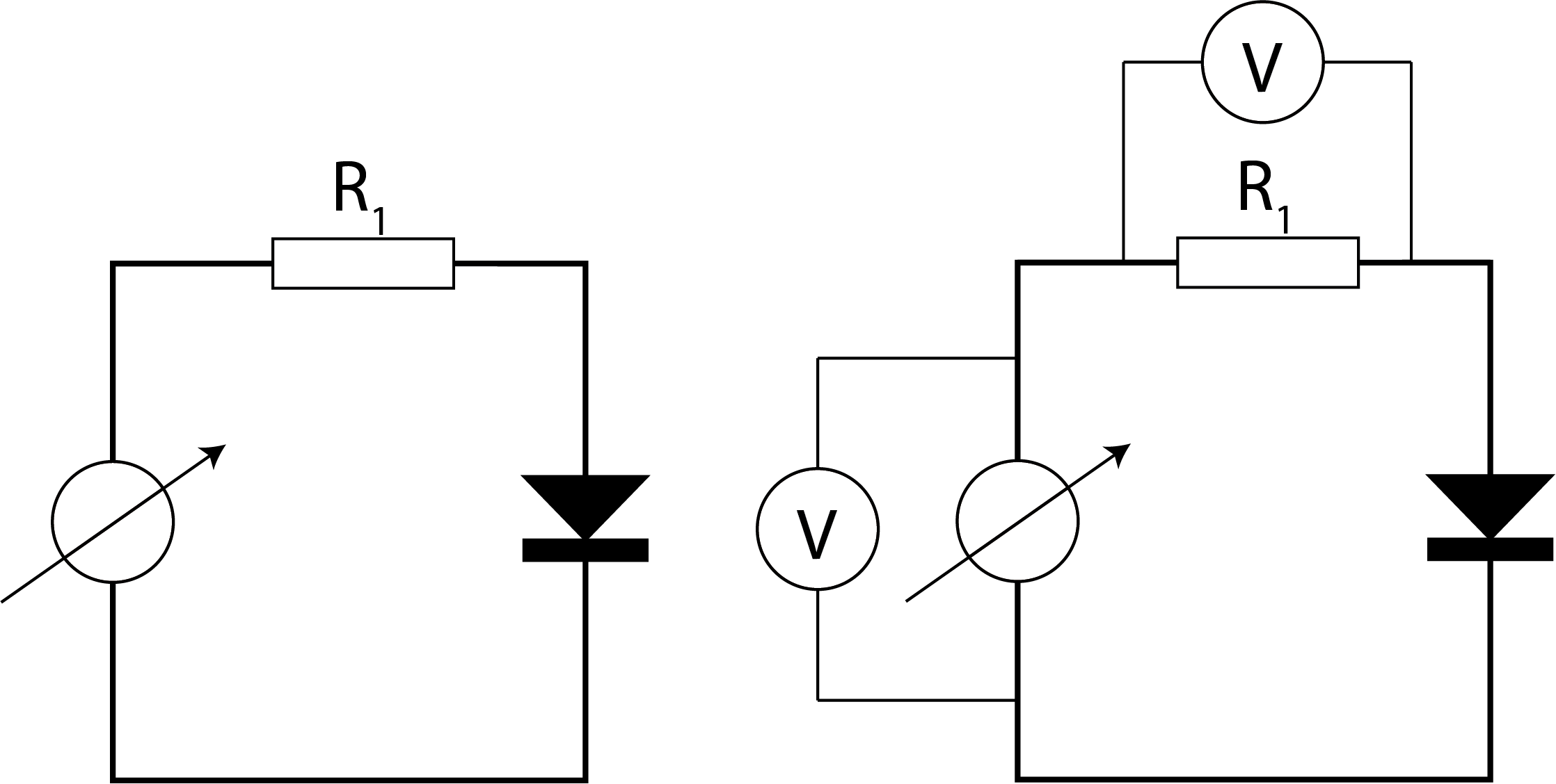
Fig. 9.1 Het meten van de spanning verandert het elektrische circuit zelf.

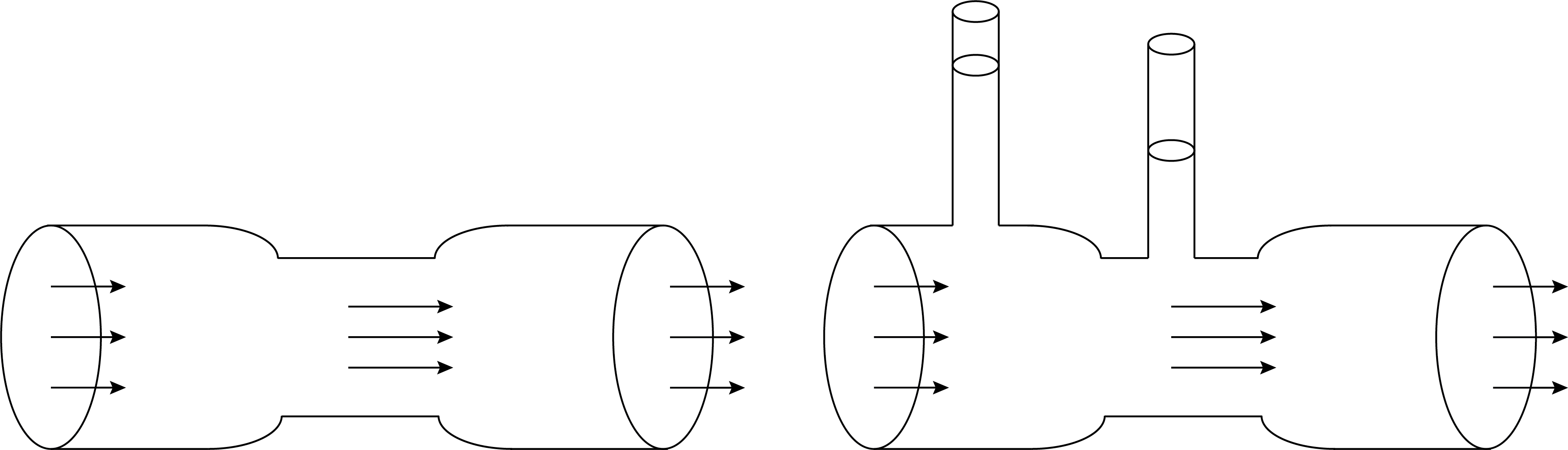
Fig. 9.2 Het plaatsen van drukmeters in een vloeistofstroom beïnvloedt de oorspronkelijke stroom.

9.6.1. Systematic error

Naast beïnvloeding van de meting aan je fysische grootheid door die te meten, zijn er andere oorzaken die kunnen leiden tot ‘fouten’. We onderscheiden daarin systematische fouten van willekeurige fouten. Een systematische fout zal altijd even groot zijn, en zorgt dus voor een afwijking in je gemiddelde resultaat. Zo’n fout beïnvloedt sterk je eindresultaat. Gelukkig kun je hier wel voor corrigeren. Voorbeelden van systematische fouten zijn een nulpuntsfout en een calibratiefout, zie bijvoorbeeld Figuur 9.3.

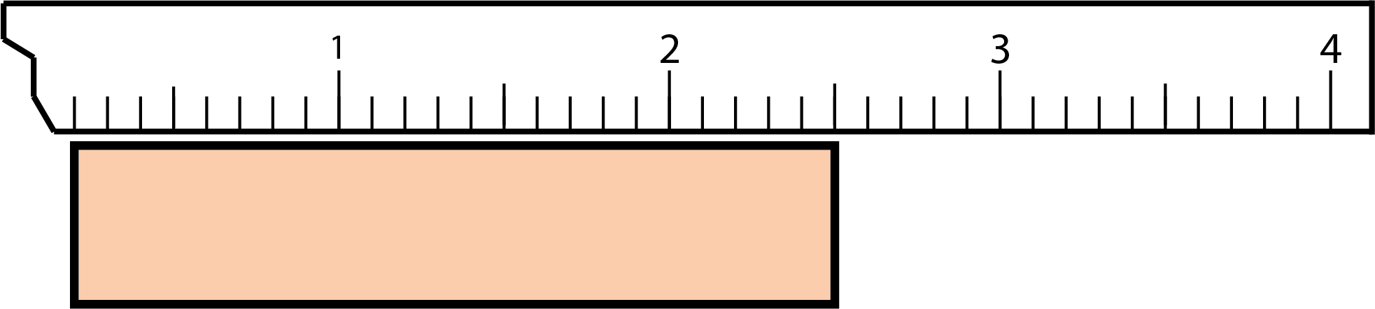
Fig. 9.3 Hier ontstaat een systematische fout wanneer je er niet op bedacht bent dat de liniaal niet bij 0 begint.

Om er achter te komen of er een systematische fout in je data zit, kun je dit controleren met bijvoorbeeld Python. Het best valt dit uit te leggen aan de hand van een voorbeeld.

Voorbeeld: Systematische fout

Je doet een onderzoek naar de invloed van de afstand op de kracht. Je meet daartoe de afstand, maar bent bang dat er sprake is van een systematische fout in de onderlinge afstand \(r\) omdat die afstand niet goed te meten is. Als je het te verwachten verband \(F = \frac{a}{r^4}\) onderzoekt, kun je proberen de functie \(F = \frac{a}{(r+\Delta r)^4}\) te fitten. In de ideale situatie, zonder systematische fout, is \(\Delta r\) gelijk aan 0. Als dit een betere fit oplevert voor \(\Delta r \neq 0\) (Figuur 9.4), dan kan \(\Delta r\) je systematische fout zijn. Natuurlijk moet je dan nog onderzoeken of deze waarde redelijk is en te verklaren valt.

In Figuur 9.4 is het verschil te zien tussen een fit met en zonder compensatie van systematische fout. Alhoewel de bovenste figuur een goede fit lijkt te zijn, is te zien dat de fit van de onderste figuur nog beter door alle metingen heen gaan. Straks zullen we bekijken hoe we zulke fouten systematischer kunnen onderzoeken.

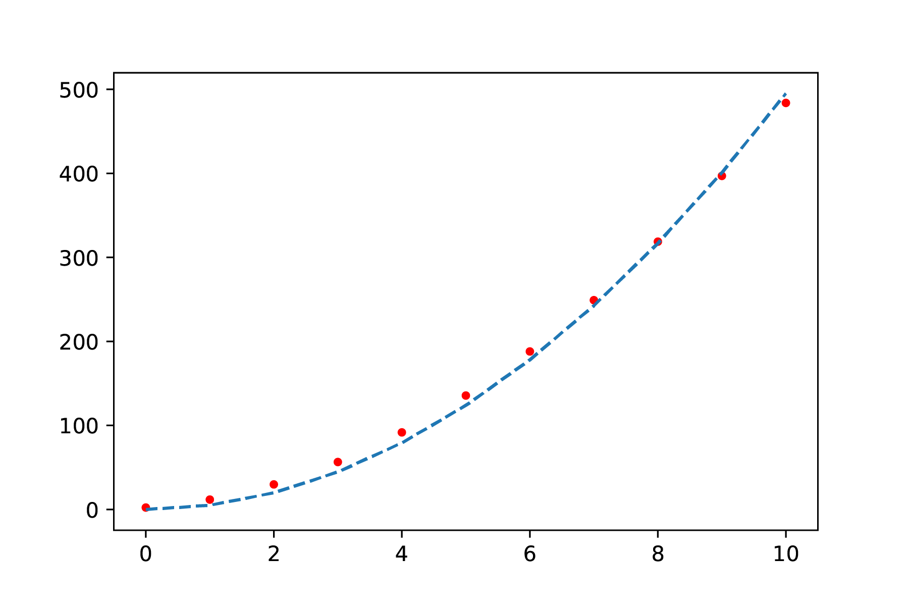
Fig. 9.4 Least-squares curve fit zonder correctie voor een systematische fout: \(F = \frac{a}{r^4}\)

Fig. 9.5 Least-squares fit met correctie voor een systematische fout: \(F = \frac{a}{(r+\Delta r)^4}\) Duidelijk is dat de fit nu door alle meetpunten gaat.

9.6.2. Random error

Een willekeurige meetfout kan ontstaan door bijvoorbeeld temperatuurschommelingen, vibraties, luchtstromingen, botsingen op moleculair niveau etc. Er is dan sprake van een technische willekeurige fout. Deze onzekerheden kun je niet altijd verkleinen. Willekeurige fouten zijn zowel positief als negatief, en middelen dus uit als je genoeg metingen doet. Je kunt er mee werken en rekenen doordat er een kansverdeling aan ten grondslag ligt. In de volgende paragrafen gaan we er van uit dat je steeds te maken hebt met een willekeurige fout, dat wil zeggen een fout die niet gecorreleerd is met andere variabelen en waarvan de kans dat die fout optreedt normaal (Gaussisch) verdeeld is.

Naast technische willekeurige fouten, kun je te maken krijgen met fundamentele fouten doordat aan sommige metingen een fysische beperking zit, bijvoorbeeld door thermische fluctuaties wanneer je meet aan stroomsterktes. Er is dan sprake van een fundamentele willekeurige fout. Deze bijdrage aan de meetonzekerheid kun je niet reduceren. De bijdrage aan de totale onzekerheid kan zowel positief als negatief zijn.

9.6.3. Instrumental uncertainties

Elk instrument dat je gebruikt heeft bepaalde beperkingen. De onzekerheid kan liggen in het aflezen van het instrument, maar ook aan het instrument zelf, en dan ook nog eens aan de waarde van de gemeten grootheid. Daarnaast moet je (sommige) instrumenten eerst ijken voordat je ze gebruikt. Een fout in de ijking kan leiden tot een systematisch fout.

Bij het gebruik van instrumenten wordt vaak gebruik gemaakt van de termen precision en accuracy. Precision verwijst naar de kleine spreiding in de metingen. Precision is nauw verbonden met willekeurige fouten. Accuracy verwijst naar hoe dicht de metingen liggen op de gewenste waarde. Accuracy is nauw verbonden met systematische fouten. De vier varianten die je kunt hebben, zijn weergegeven in Figuur 9.6.

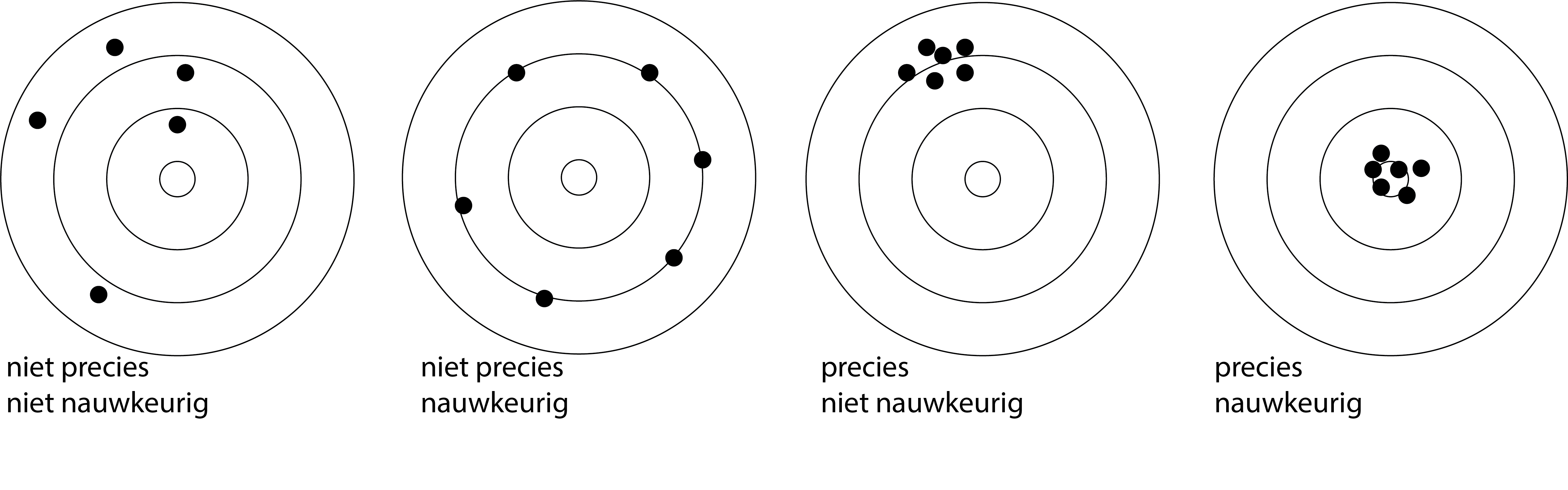
Fig. 9.6 De vier varianten aangaande nauwkeurigheid en precisie. Nauwkeurigheid is sterk gelinkt aan systematische fouten, precisie aan willekeurige fouten.

Note

Meetschalen De verschillende meetinstrumenten hebben verschillende meetschalen. We onderscheiden een nominale, een ordinale, een interval, een ratio en een kardinale schaal.

1. Nominale schaal
Als we alleen de kwaliteit van het object benoemen, dan heet de meetschaal nominaal. Vaststellen van de kleur van een oplossing is daarvan een voorbeeld.

2. Ordinale schaal
Als de benoeming een rangordening inhoudt, spreken we van een ordinale schaal. Een voorbeeld is het geven van cijfers voor studieprestaties. Iemand met een 10 weet meer dan iemand met een 5, maar zo iemand weet niet twee keer zoveel. Ook is het verschil in kennis tussen een 5 en een 6 meestal onvergelijkbaar met het verschil tussen een 9 en een 10.

3. Intervalschaal
Een schaal waarop gelijke verschillen wel hetzelfde betekenen maar verhoudingen niet, heet een intervalschaal. Op een intervalschaal is het nulpunt willekeurig. De Celsiusschaal is daarvan een voorbeeld. 100 ˚C is niet een twee keer zo hoge temperatuur als 50 ˚C, maar wel is het temperatuurverschil tussen 50 ˚C en 51 ˚C hetzelfde als tussen 100 ˚C en 101 ˚C.

4. Ratioschaal
Als we behalve met verschillen ook met verhoudingen (ratio’s) van meetuitkomsten zinvol kunnen rekenen, dan vindt de meting plaats op ratioschaal. Meten van lengtes is een voorbeeld. Een tafel van 2m breed is twee keer zo breed als een tafel van 1m. We streven er naar het meten op het niveau van een ratioschaal te brengen. Een voorbeeld is het overgaan van de Celsiusschaal op de absolute temperatuurschaal (de Kelvinschaal).

5. Kardinale schaal
Het feit dat we op een intervalschaal met vastgelegd nulpunt of op een ratioschaal kunnen meten legt de getalwaarden niet vast. Pas als we de eenheid hebben gekozen (voor Celsiustemperaturen de ˚C, voor lengtes bijvoorbeeld de meter), kunnen we getalwaarden toekennen. We spreken dan van een kardinale schaal.

Meetonzekerheid bij analoge instrumenten
Bij analoge instrumenten moet je aflezen wat de waarde is, zie Figuur 9.7. In sommige gevallen zit er achter de wijzer een spiegeltje zodat je niet al een fout maakt door de wijzer onder een hoek af te lezen. Daarnaast kun je niet oneindig precies aflezen wat de waarde is. Denk aan meetlat waar je op mm nauwkeurig kunt meten, maar afstanden tussen de mm niet goed te bepalen zijn, zeker niet wanneer de lijntjes van het liniaal dik zijn. Voor het aflezen van een analoge meter moet je een inschatting maken van de bijbehorende onzekerheid:

• Lees de waarde zo goed mogelijk af.

• Bepaal de waarden die je nog goed kunt aflezen.

• Neem vervolgens de helft van de waarde die je tussen twee nog te bepalen waarden als maat voor onzekerheid.

Voorbeeld: Interpoleren van afgelezen waarde

De beste aflezing van de wijzer in Figuur 9.7 zou 17.3 zijn. De waarde ligt duidelijk tussen 17 en 17.5, dichter bij de 17.5 dan de 17. De waarden 17 en 17.5 zou je goed kunnen aflezen. De helft van daarvan is 0.25. De onzekerheid is dan 0.3 (we mogen een onzekerheid niet naar beneden afronden).

Zoals je ziet zijn er lang niet altijd vaste voorgeschreven regels voor het bepalen van de meetonzekerheid en komt het soms neer op gezond verstand en beargumenteren hoe je aan die waarde komt.

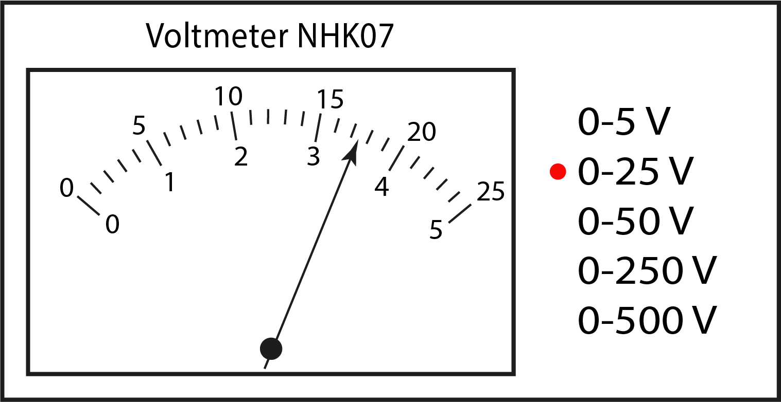
Fig. 9.7 Het aflezen van een analoge meter waarbij het eerste decimaal op basis van interpolatie geschat moet worden.

Meetonzekerheid bij digitale instrumenten
Bij het aflezen van een digitaal instrument, zie Figuur 9.8 zou je zeggen dat de onzekerheid zit in het laatste decimale cijfer dat getoond wordt. Echter is de onzekerheid van digitale instrumenten veel groter dan het laatste decimale cijfer, denk maar eens aan de onzekerheid bij het gebruik van een stopwatch. Bij apparaten die je op het natuurkundig practicum gebruikt, wordt die onzekerheid soms zelfs bepaald door de leeftijd van het apparaat en de tijd dat deze aanstaat (warm worden). Voor veel digitale (dure) apparaten staat in de specificaties precies vermeld hoe de meetonzekerheid berekend moet worden.

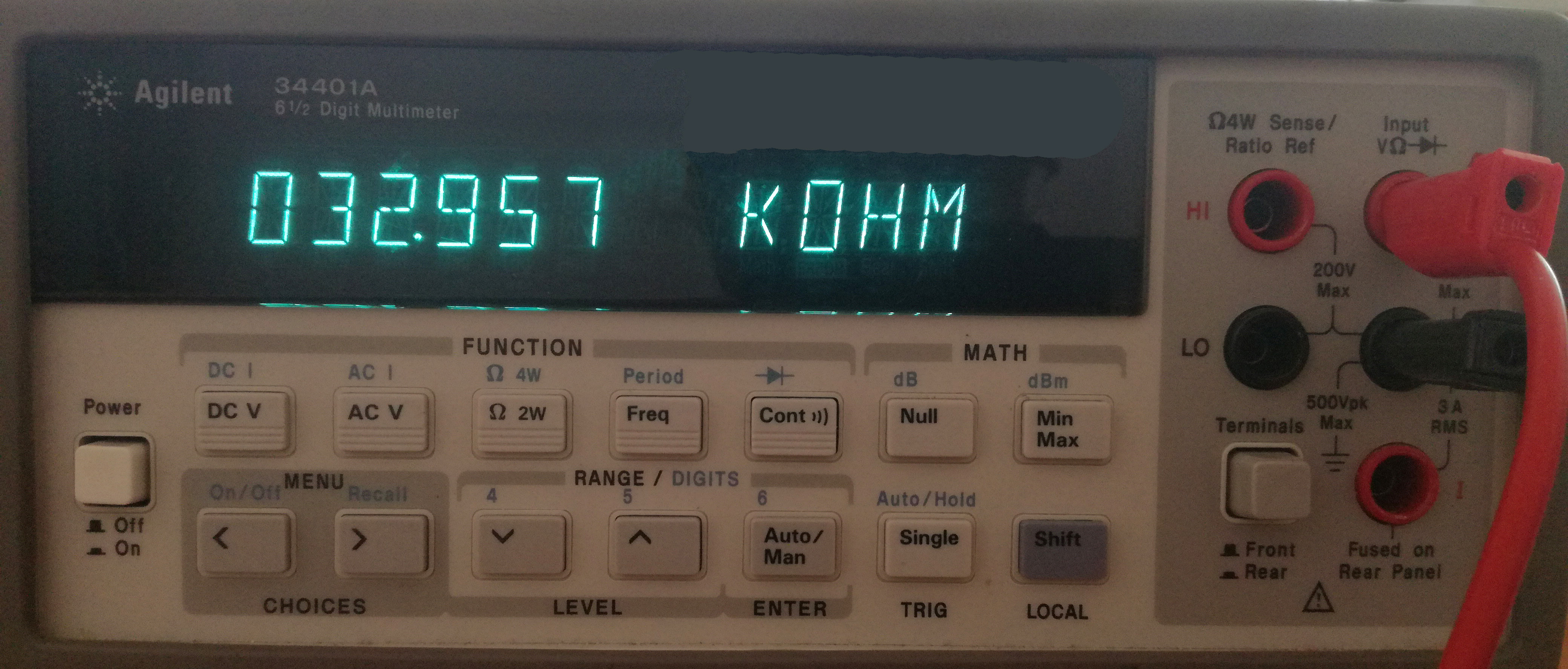
Fig. 9.8 De digitale multimeter bepaalt de ’exacte’ waarde van een 33 kΩ (5% tolerantie) weerstand

9.7. Mean, standard deviation and standard error

Doordat meetwaarden kunnen fluctueren, geeft het gemiddelde van een serie herhaalde metingen (\(x_i\)) de best mogelijke benadering van de werkelijke waarde. De gemiddelde waarde bereken je op basis van de serie herhaalde metingen:

(9.1)\[\mu(x)=\overline{x} = \frac{x_1 + x_2 + x_3 + ... + x_n}{N} = \frac{1}{N}\sum_{i=1}^{N} x_i\]

Uiteraard is een herhaalde meting alleen zinnig wanneer je instrument nauwkeurig genoeg is om variaties te tonen. In de serie metingen zit een mate van spreiding: De metingen verschillen van elkaar. De standaard deviatie is een maat voor die spreiding:

(9.2)\[\sigma(x) = \sqrt{\frac{\sum_{i=1}^N (x_i-\overline{x})^2}{N-1}}\]

Alhoewel het gemiddelde en de standaard deviatie beter gedefinieerd worden met meer metingen, neemt de standaard deviatie niet af in waarde, zie Figuur 9.9. De spreiding zelf is dan ook geen goede maat voor de onzekerheid in je gemiddelde waarde. De onzekerheid in je gemiddelde wordt gegeven door:

(9.3)\[u(x) = \frac{\sigma(x)}{\sqrt{N}}\]

Een belangrijk inzicht is dat de meetonzekerheid afneemt met de wortel van het aantal metingen. Om de meetonzekerheid op basis van meerdere metingen 10x zo klein te krijgen, moet je 100x zoveel herhaalde metingen uitvoeren. Het optimum van het aantal herhaalde metingen hangt dan ook af van (1) de nauwkeurigheid die je wilt hebben, en (2) de tijd en geld die je hebt om die nauwkeurigheid te verkrijgen.

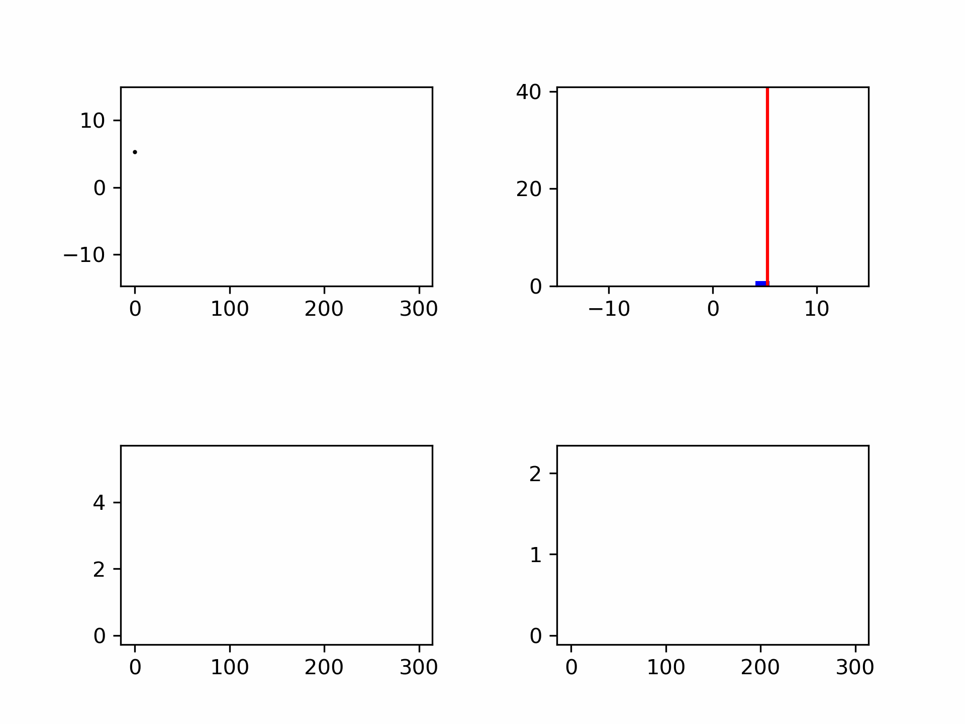
Fig. 9.9 Het genereren van ruis weergegeven als punten en in een histogram. Links onder de standaard deviatie (convergeert) en rechtsonder de meetonzekerheid (wordt kleiner met \(\frac{1}{\sqrt{N}}\)).

De meetonzekerheid is gelijk aan de deviatie van het gemiddelde van herhaalde experimenten. Dat wil zeggen, als het volledige experiment herhaald wordt, zal er steeds een verschil zitten in het gevonden gemiddelde. De standaard deviatie daarvan is gelijk aan \(u(x)\), ofwel, er is een kans van grofweg 2/3 dat bij een herhaling van het volledige experiment het gemiddelde tussen \(\overline{x} \pm u(x)\) ligt. In onderstaande code zie je hoe je die bewering zou kunnen controleren.

Tip

Om de code hieronder te runnen en aan te passen, druk op het raketje bovenaan de pagina. Na het inladen van de benodigde packages, kun je aan de slag!

De uiteindelijke waarde die je gebruikt noteer je als:

\[ Meting \pm onzekerheid + eenheid \]

De onzekerheid bepaalt het aantal te gebruiken significante cijfers. Je gebruikt namelijk hetzelfde aantal decimale cijfers.

Voorbeeld: Notatie

Het gemiddelde van een herhaalde meting is 4.04 V met een onzekerheid van 0.1 V. De onzekerheid heeft 1 decimaal getal, de meting noteer je dan als: (4.0 \(\pm\) 0.1) V.

Exercise 9.2

Bepaal het gemiddelde, standaardafwijking en standaardfout van de volgende meetseries:

1. 0.10; 0.15; 0.18; 0.13

2. 25; 26; 30; 27; 19

3. 3.05; 2.75; 3.28; 2.88

Solution to Exercise 9.2

1. \(\overline{x}\)=0.14, \(\sigma\) = 0.034, \(u\) = 0.02

2. \(\overline{x}\)=25.4, \(\sigma\) = 4.0, \(u\) = 2

3. \(\overline{x}\)=2.99, \(\sigma\) = .23, \(u\) = 0.1

9.7.1. Weighted average

Het kan voorkomen dat niet alle herhaalde metingen even betrouwbaar zijn. Als meting 1 twee keer zo kleine onzekerheid heeft als meting 2, dan lijkt het logisch dat het gemiddelde berekend wordt door \(\frac{2 \cdot x_1 + 1 \cdot x_2}{3}\). We spreken dan over een gewogen gemiddelde. De vraag is dan natuurlijk hoe je aan de uitspraak komt over de betrouwbaarheid en hoe we daarmee aan onze weegfactor komen. Gelukkig hebben we daar net een maat voor gevonden, nl. de meetonzekerheid. De weegfactor wordt gedefinieerd door:

(9.4)\[w_i = \frac{1}{u(x_i)^2}\]

Het gewogen gemiddelde is daarmee:

(9.5)\[\overline{x} = \frac{w_1 x_1 + w_2 x_2 + w_3 x_3 + ... + w_n x_n}{w_1 + w_2 + w_3 + ... + w_n} = \frac{\sum_{i=1}^{N} w_i x_i}{\sum_{i=1}^{N} w_i}.\]

met een bijbehorende onzekerheid van:

(9.6)\[u(x) = \sqrt{\frac{1}{\sum_i^N{w_i}}}\]

Merk op dat de bovenstaande formule wordt gereduceerd tot het normale gemiddelde als alle weegfactoren \(w_i\) gelijk zijn aan 1.

Exercise 9.3

In een experiment bij het natuurkundig practicum wordt de valversnelling bepaald. Dit levert de volgende waarden op bij verschillende groepjes: 9.814 ± 0.007, 9.807 ± 0.003, 9.813 ± 0.004.

Bereken het gewogen gemiddelde en de bijbehorende onzekerheid.

Solution to Exercise 9.3

9.809 ± 0.002 m/s²

Merk op dat de onzekerheid in het eindantwoord kleiner is geworden!

9.8. Probability distributions

Zoals aangegeven zit er spreiding in herhaalde metingen. De fysische meting \(M\) kunnen we zien als de optelsom van de fysische waarde \(G\) en ruis \(s\):

(9.7)\[M = G + s\]

Ruis is hier ruim gedefinieerd, we verstaan er hier even alle mogelijke fouten onder. Onze interesse gaat met name uit naar willekeurige fouten. Deze zijn normaal verdeeld.

9.8.1. Gaussian distribution

Wanneer we te maken hebben met willekeurige ruis, dan kan de kans dat een waarde optreedt beschreven worden aan de hand van een normale (Gaussische) verdeling:

(9.8)\[ P(x) = \frac{1}{{\sigma \sqrt{2\pi}}}e^{\frac{{-(x - \mu)^2}}{{2\sigma^2}}} \]

hierin is \(P(x)\) de kansdichtheidsfunctie, met \(\mu\) het gemiddelde waarde van de ruis en \(\sigma\) de standaard deviatie.

Een voorbeeld van een ruis signaal is weergegeven in Figuur 9.10 (de bijbehorende code is in een cel daaronder getoond). Het gemiddelde van deze waarden is 0. Het herhalen van metingen zorgt er dus voor dat de invloed van de ruis beperkt wordt omdat de gemiddelde bijdrage 0 is:

(9.9)\[\overline{M} = \frac{\sum_{i=1}^{N} (G + s)}{N} = \frac{\sum_{i=1}^{N} G + \sum_{i=1}^{N} s}{N} = \frac{\sum_{i=1}^{N} G}{N} = \overline{G}\]

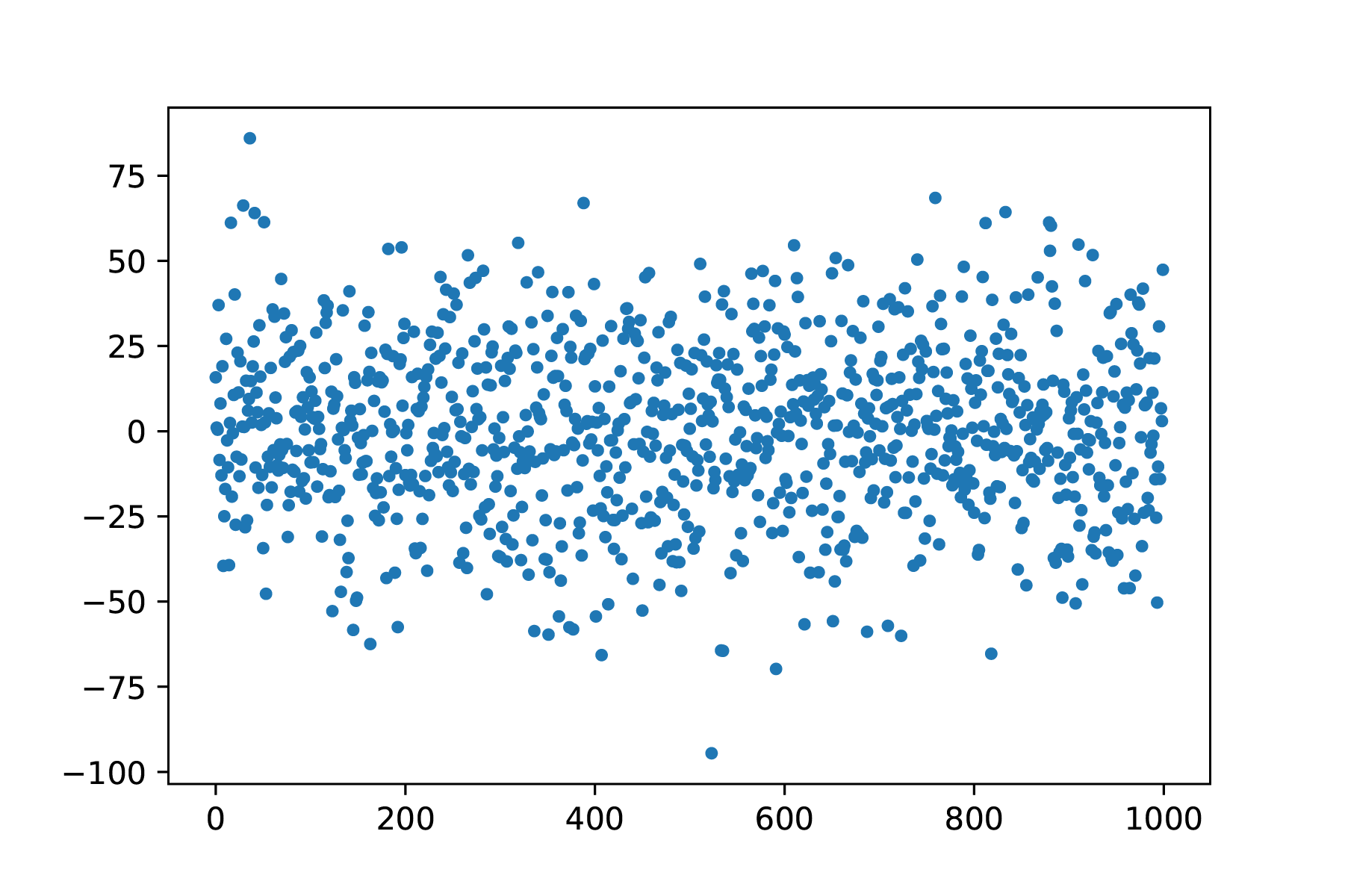
Fig. 9.10 Random noise, te zien is dat grote uitschieters voorkomen, maar minder frequent.

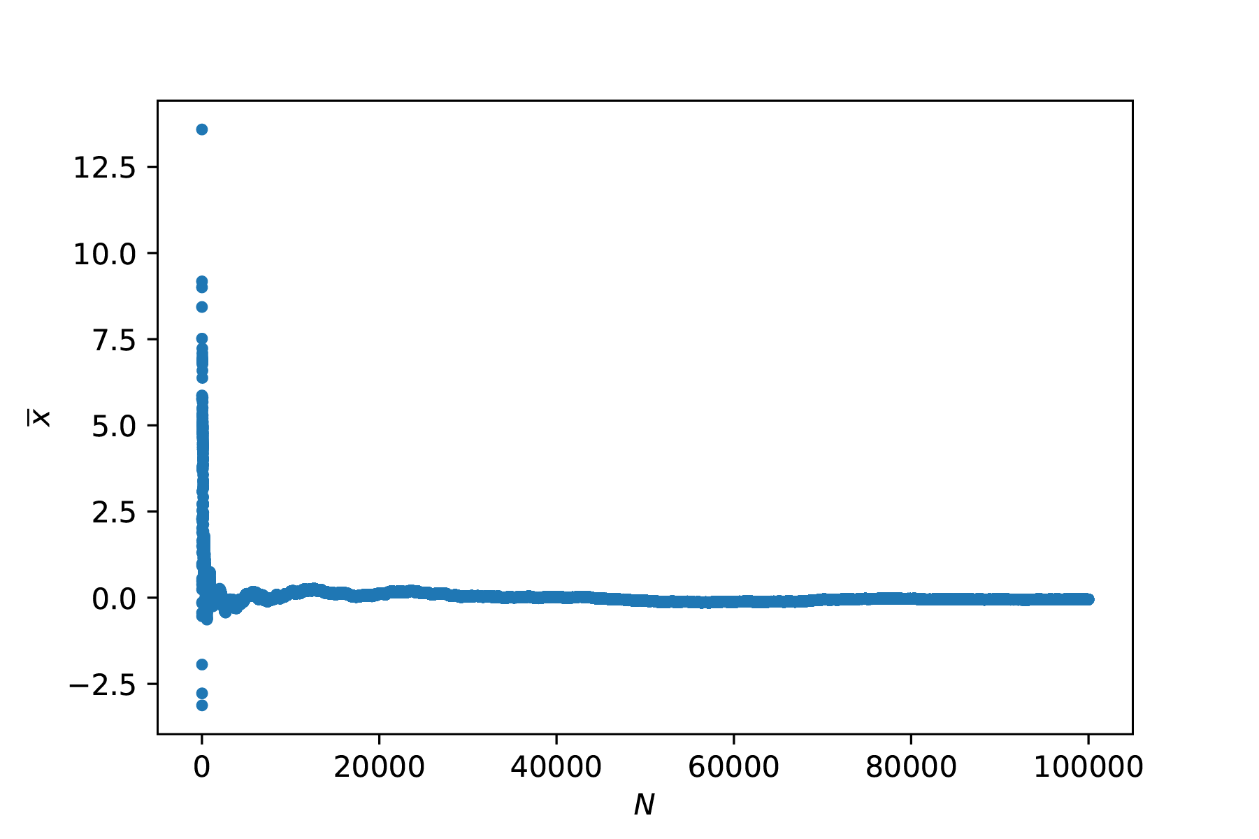
Fig. 9.11 De gemiddelde waarde van ruis wordt steeds beter gedefinieerd bij herhaalde metingen.

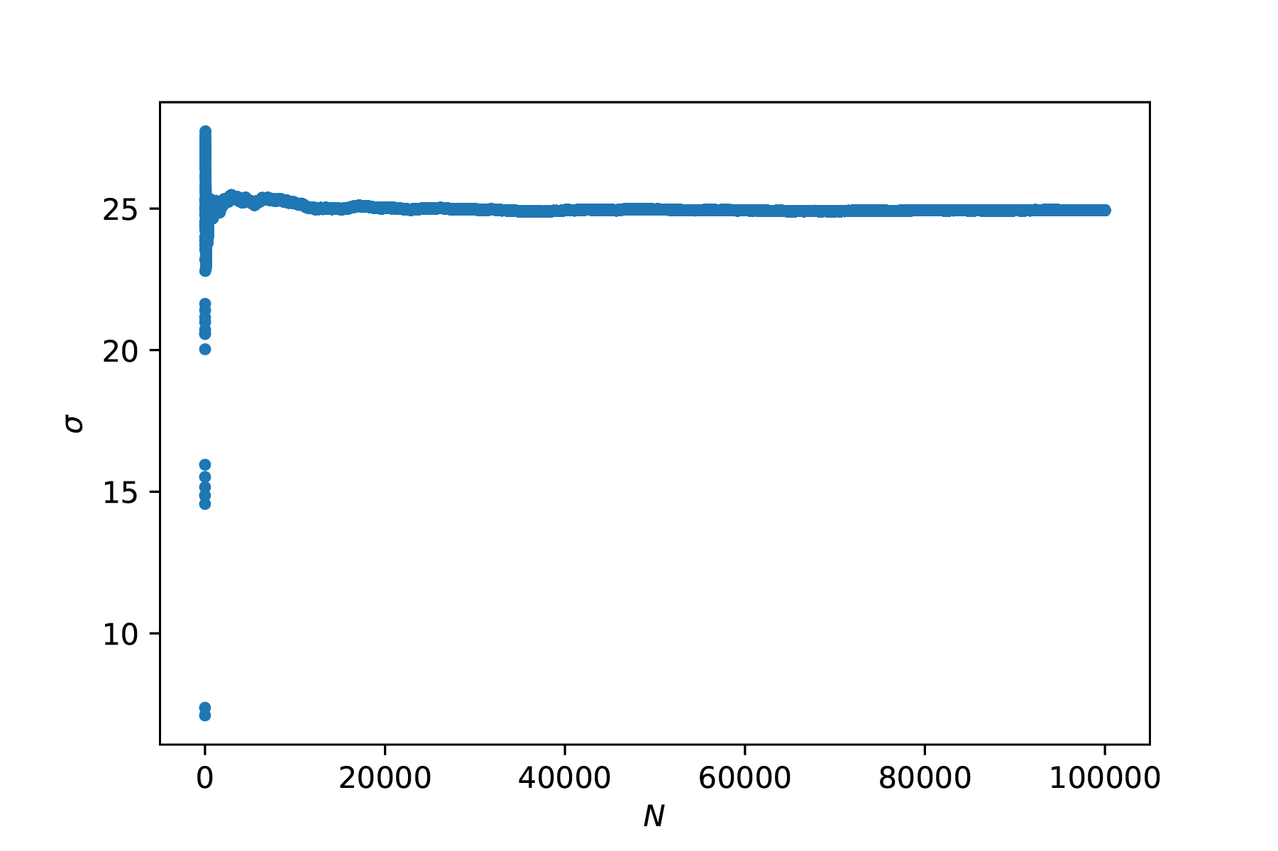
Fig. 9.12 De standaard deviatie wordt steeds beter gedefinieerd bij herhaalde metingen.

We moeten hier wel voorzichtig mee zijn, in Figuur 9.13 is te zien dat een histogram van vier herhaalde metingen aan ruis steeds een net iets ander beeld geeft. Elk histogram bestaat uit een 1000 herhaalde metingen. Er is dus zelfs een onzekerheid in de onzekerheid \(\left( \frac{1}{\sqrt{2N-2}}\right )\). De precieze wijze waarop we onze waarden rapporteren is uitgewerkt in Standaard onzekerheid en significante cijfers.

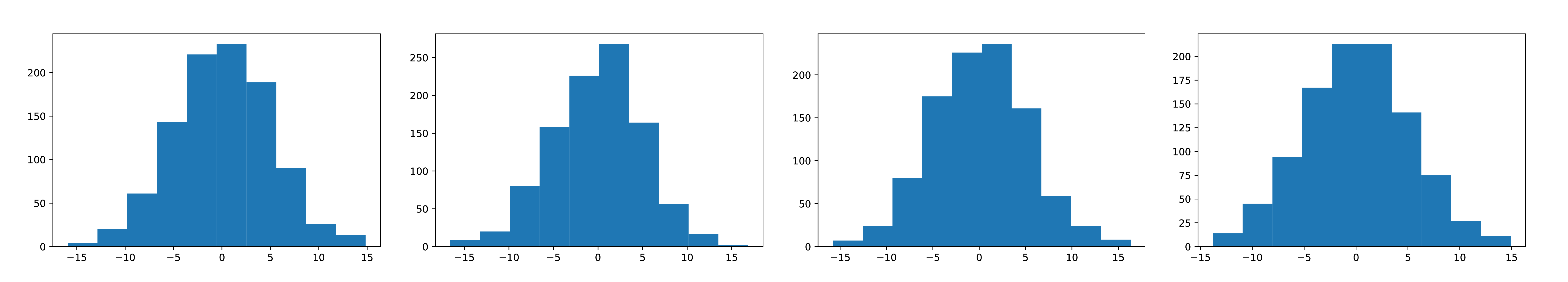
Fig. 9.13 Zelfs 1000 herhaalde metingen (aan ruis) laten verschillen zien.

import matplotlib.pyplot as plt
import numpy as np
from scipy.optimize import curve_fit 
from scipy.stats import norm, poisson

# Maken van 1000 random punten
x = np.random.normal(0,5,1000)

# Bereken van gemiddelde waarde en standaard deviatie
av_x = np.array([])
std_x = np.array([])
for i in range(1,len(x)-1):
    av_x = np.append(av_x,np.mean(x[:i]))
    std_x = np.append(std_x,np.std(x[:i],ddof=1))

# Plotten van de waarden als functie van N
fig, axs = plt.subplots(1,3,figsize=(15, 5))
axs[0].plot(x,'k.',markersize=1)
axs[0].set_xlabel('N')
axs[0].set_ylabel('')

axs[1].plot(av_x,'k.',ms=1)
axs[1].set_xlabel('N')
axs[1].set_ylabel('average of x as function of N')

axs[2].plot(std_x,'k.',ms=1)
axs[2].set_xlabel('N')
axs[2].set_ylabel('standard deviation of x as function of N')

plt.show()

# we voeren hier een experiment met 1000 samples 100x uit. Als bovenstaande klopt, dan is de standaard deviatie in het gemiddelde van de verschillende experimenten gelijk aan de onzekerheid in een enkele dataset.


mean_values = np.array([])
N = 100
samples = 1000

for i in range(N):
    dataset = np.random.normal(1.00,0.5,samples) 
    mean_values = np.append(mean_values,np.mean(dataset))
    
print('De standaard deviatie in het gemiddelde van herhaalde experimenten is: ', np.std(mean_values,ddof=1))
print('De onzekerheid in een enkele dataset is: ', np.std(dataset,ddof=1)/np.sqrt(samples))

9.8.2. Poisson distribution

Een tweede kansverdeling die we hier introduceren is de Poissonverdeling. De Poissonverdeling is een discrete (in tegenstelling tot de normaalverdeling) kansverdeling, die gebruikt wordt om onafhankelijke gebeurtenissen te tellen binnen een bepaalde tijd, waarbij de evenementen zelf ook op een normale verdeling zijn gebaseerd. Voorbeelden hiervan zijn radioactief verval, het aantal fotonen dat op een detector valt, etc.

De kans op \(k\) gebeurtenissen binnen een bepaalde tijd met een gemiddelde van \(\lambda\) wordt gegeven door:

(9.10)\[ P(X = k) = \frac{\lambda^k e^{-\lambda}}{k!}. \]

De standaardafwijking in een Poissonverdeling is gelijk aan de wortel van het gemiddelde (\(\sigma = \sqrt{\lambda}\)).

Voorbeeld: Poisson

In een restaurant komen dagelijks gemiddeld 20 mensen eten. Hoe ziet de kansverdeling van het aantal mensen dat komt eten er uit?
De kansverdeling van het aantal bezoekers is weergegeven in Figuur 9.14 De kans wordt beschreven door: \(P(X = k) = \frac{20^k e^{-20}}{k!}\).

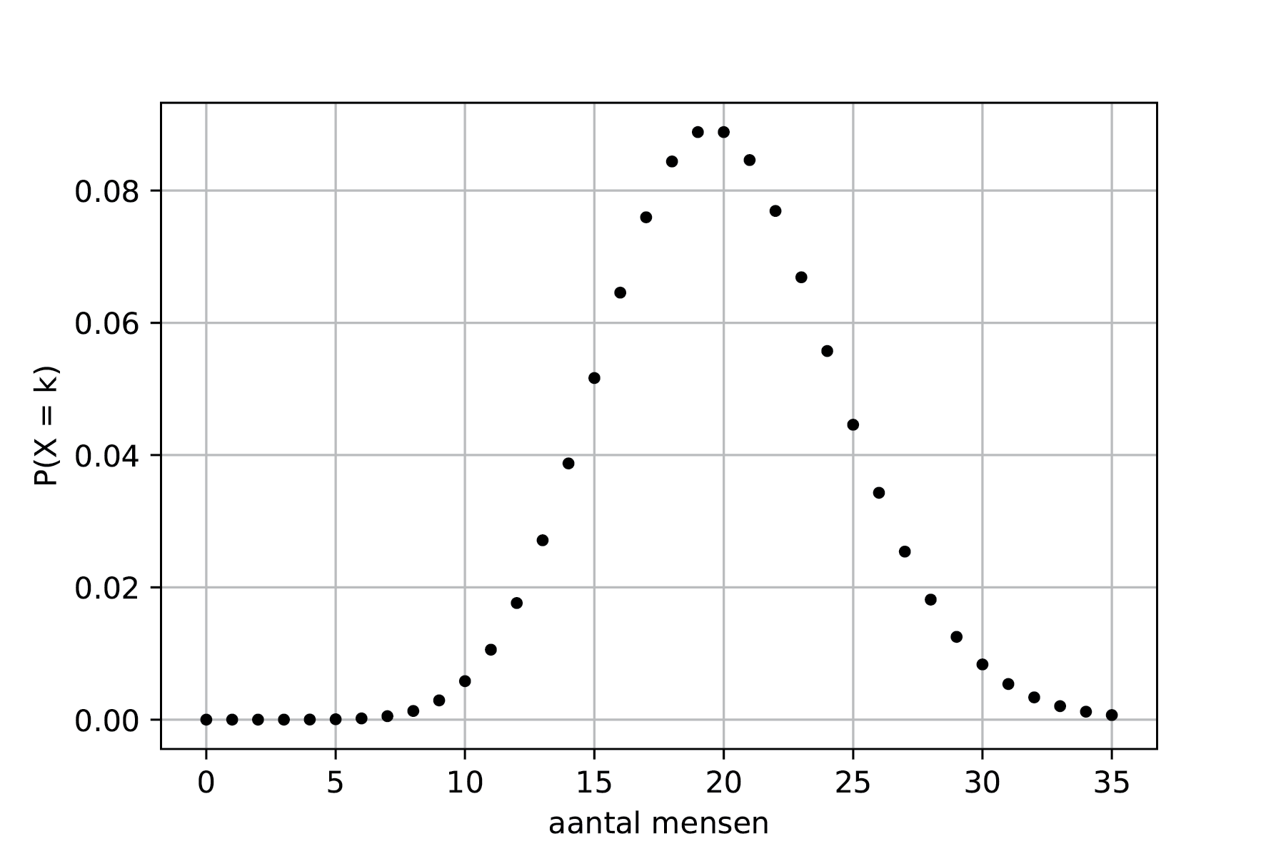
Fig. 9.14 De kansverdeling van het aantal bezoekers van het restaurant.

Zowel de vorm als de functie lijken wat op die van de Gaussische verdeling. Maar met name bij kleine waarden voor \(\lambda\) zijn er duidelijke verschillen. Ook is het aantal events altijd groter dan 0, terwijl bij een Gaussische verdeling een verwachtingswaarde ook kleiner kan zijn dan 0.

9.8.3. Uniform distribution

Als je een dobbelsteen gooit is de kans op het gooien van een 1 even groot als het gooien van een 6. Met andere woorden, de kans voor willekeurig welk getal is uniform (discreet) verdeeld. Stel nu dat we te maken hebben met een continue, uniforme kansverdeling dan geldt er voor de kansdichtheidsfunctie:

(9.11)\[\begin{split} P(x)= \begin{cases} \frac{1}{b-a},& \text{als } a<x<b\\ 0, & \text{elders} \end{cases} \end{split}\]

De kans dat een punt zich tussen de waarde \(X\) en \(X+dX\) bevindt (als \(X\) zich tussen \(a\) en \(b\) bevindt!), wordt dan gegeven door:

\[ p(X<x<X+dX) = \int_{X}^{X+dX}\frac{1}{b-a}dx \]

De verwachtingswaarde is eenvoudig uit te rekenen en wordt gegeven door:

(9.12)\[ \mu = \frac{a+b}{2} \]

en de standaard deviatie:

(9.13)\[ \sigma = \sqrt{\frac{(b-a)^2}{12}} \]

9.8.3.1. Monte Carlo simulation

Zo’n uniforme verdeling is handig bij bijvoorbeeld Monte Carlo simulaties. In zo’n simulatie wordt een groot aantal random punten aangemaakt en vervolgens wordt onderzocht waar die punten terecht komen. Voor een niet analytische oplosbare integraal kun je zo alsnog het oppervlak uitrekenen, nl:

(9.14)\[ \int_{a}^{b} f(x) dx = \frac{N}{N_{totaal}} \cdot (b-a) \cdot (y_{max} - y_{min}) \]

Hierin zijn \(y_{min}\) en \(y_{max}\) de verticale grenzen die je kiest voor het maken van je random punten. Die moeten natuurlijk wel de gehele grafiek omvatten!

Een voorbeeld van een Monte Carlo simulatie is gegeven in Figuur 9.15 waarbij een eenvoudige integraal is uitgerekend door voor 10.000 punten uit te rekenen of geldt: \(y<x^2\). De integraal op het domein [0,5] is dan gelijk aan het aantal punten dat aan deze voorwaarde voldoet gedeeld door het totaal aantal gecreëerde punten maal 5 maal 25. In zo’n Monte Carlo simulatie (wat een telprobleem is) schaalt de onzekerheid met \(\frac{1}{\sqrt{N}}\), waarin \(N\) het aantal punten is dat voldoet aan de voorwaarde (dus kies je de verticale grenzen optimaal!).

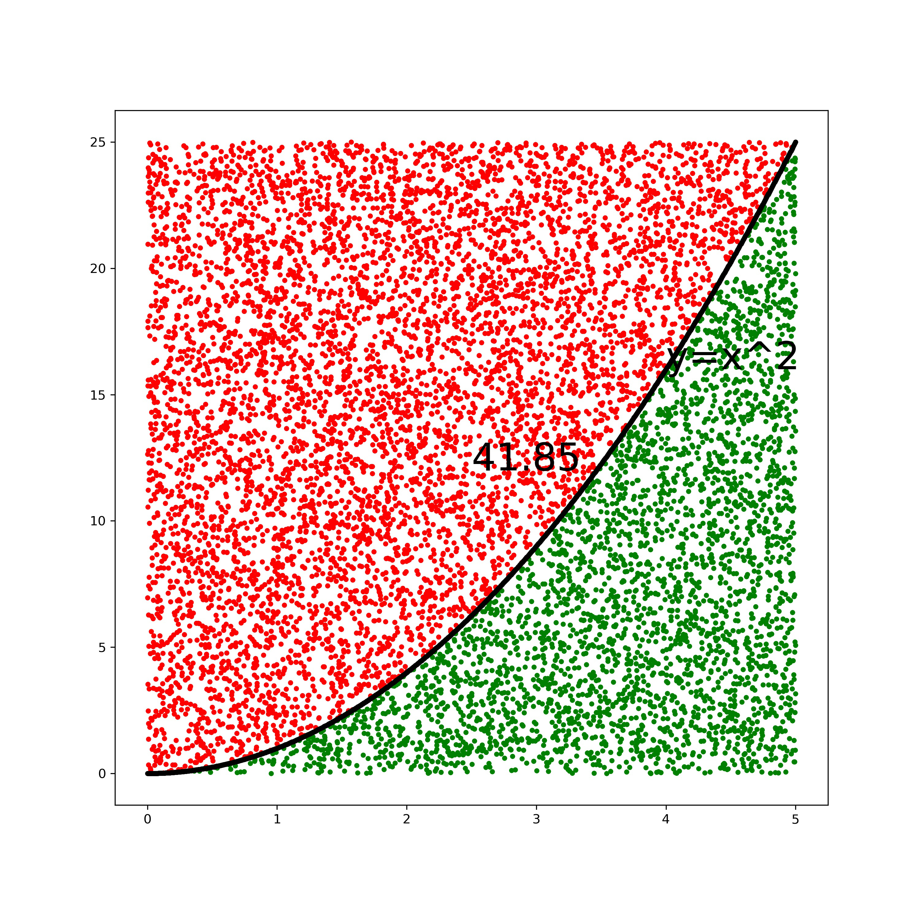
Fig. 9.15 Een voorbeeld van een Monte Carlo simulatie voor het berekenen van een integraal met behulp van een uniforme verdeling van random punten.

9.8.4. Chauvenet’s criterium

Herhaalde metingen leiden tot een beter gemiddelde. Echter in herhaalde metingen kunnen bepaalde waardes veel afwijken van het gemiddelde. Het kan verleidelijk zijn om een meetpunt dat wel erg veel afwijkt van de rest simpelweg af te schrijven als meetfout. Echter is dit al snel manipuleren van data en dat is niet de bedoeling. Je kunt het criterium van Chauvenet toe passen om te kijken of het meetpunt verwijderd mag worden. Het criterium van Chauvenet is een vuistregel (er zijn andere, meer gecompliceerde methoden om na te gaan of je datapunten mag verwijderen, maar die werken we hier niet uit). Het criterium van Chauvenet zegt dat een meting uit de dataset verwijderd mag worden als de kans daarop kleiner is dan \(\frac{1}{2N}\) ofwel \(P(X)<\frac{1}{2N}\).

Verder uitgewerkt houdt dit in dat je eerst het gemiddelde en de standaardafwijking uitrekent van je data, inclusief het verdachte punt. Vervolgens mag je een punt achterwege laten als het voldoet aan de volgende ongelijkheid:

(9.15)\[ N\cdot P_{out} < 0.5 \]

waar

(9.16)\[P_{out}=2Erf(x_{out},\overline{x},\sigma)\]

erf is hier de errorfunctie, de integraal van de normale verdeling. De uitkomst van deze integraal is niet algebraïsch uit te rekenen. Op https://www.danielsoper.com/statcalc/calculator.aspx?id=53 kun je de waarde voor de errorfunctie berekenen. Hieronder werken we uit hoe dat gaat in Python.

Als je het criterium van Chauvenet gebruikt om een outlier uit te sluiten, moet je dit altijd vermelden in je verslag! Daarnaast moet je wederom het gemiddelde en standaard deviatie uitrekenen na de verwijdering van het verdachte punt. Dit punt heeft immers een significant effect op je dataset

Exercise 9.4 (Outlier)

Welke meting uit de serie 1b is verdacht? Gebruik het criterium van Chauvenet om te kijken of je deze meting mag uitsluiten.

Solution to Exercise 9.4 (Outlier)

\(P_{out} = 2\cdot \text{Erf}(x = 19,\overline{x} = 25.4,\sigma = 4.0) = 2 \cdot 0.05479929\)

\(N\cdot P_{out} = 0.5479929 > 0.5\). We mogen het punt dus niet uitsluiten.

9.8.4.1. Error function(s)

Er zijn twee soorten error functies, de \(\text{erf}(x)\) en de \(\text{Erf}(x_{out},\overline{x},\sigma)\) (ook wel de cdf functie genoemd). Die als volgt gedefinieerd zijn:

(9.17)\[\begin{split} \begin{align*} \text{erf}(x) &= \frac{2}{\sqrt{\pi}} \int_0^x e^{-t^2} dt \\ \text{Erf}(x, \overline{x}, \sigma_x) &= \frac{1}{2} \left[1 + \text{erf}\left(\frac{x - \overline{x}}{\sqrt{2}\sigma_x}\right)\right] \end{align*} \end{split}\]

Een plot van beide is te zien in Figuur 9.16

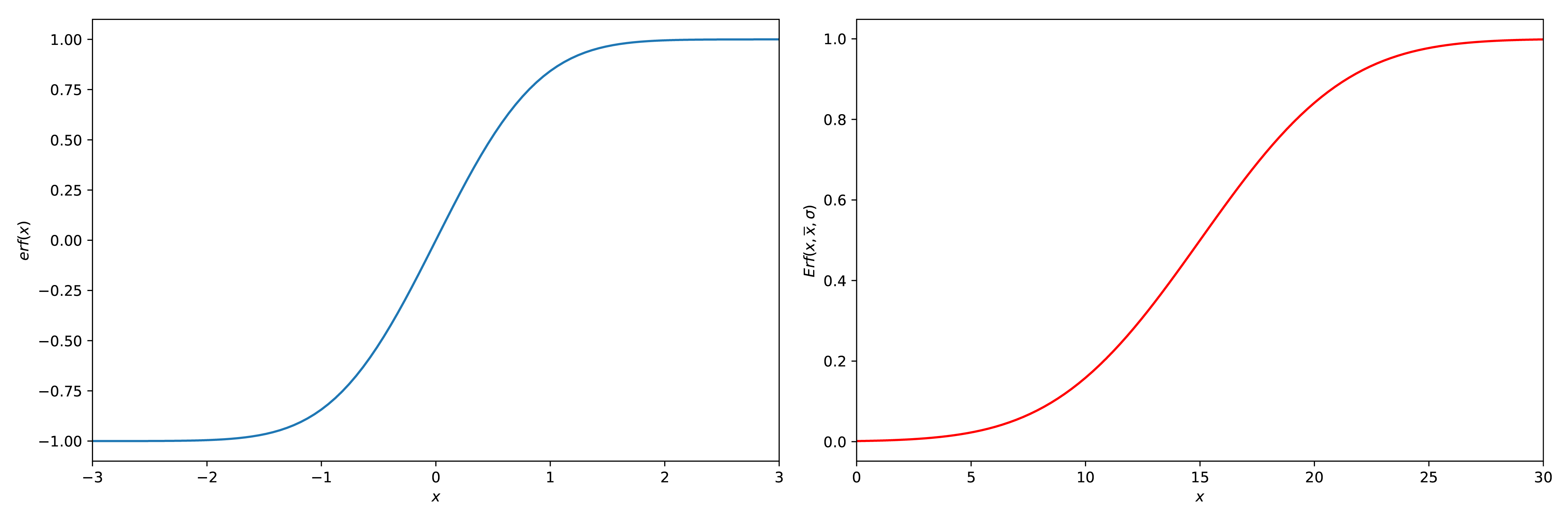
Fig. 9.16 2 plots, een met de \(\text{erf}(x)\) en een met de \(\text{Erf}(x_{out},\overline{x},\sigma)\) (rechts), \(\overline{x} = 10\) en \(\sigma = 5\).

Beide functies zijn te vinden in de scipy.special.erf en de scipy.stats.norm.cdf functie. Wanneer je gebruik maakt van de \(\text{Erf}\) of de scipy.stats.norm.cdf functie (of de site) moet je opletten dat wanneer je een outlier naar boven gaat onderzoeken dat de functies je allemaal een waarde boven de 0.5 gaan terug geven. Dit betekent dus dat je \(P_{out\_new} = 1 - P_{out}\) moet doen. De uiteindelijke code zou dus iets in deze trant moeten zijn:

from scipy.stats import norm

#P is the dataset (a numpy array)
x_out = np.max(P) #In this case, could also have been other outliers
x_mean = np.mean(P)
x_std = np.std(P,ddof=1)

#Use the Erf function
Q = norm.cdf(x_out,x_mean,x_std)

#You could have also defined the Erf on your own

#Check if it is a high 'outlier'
if Q > 0.5:
    Q = (1-Q)

#Use Chauvenets criterion
C =  2 * len(P) * Q

if C < 0.5:
    print('The value can be discarded.')
else:
    print('The value cannot be discarded.')

9.8.5. Standaard onzekerheid en significante cijfers

Een belangrijke regel met betrekking tot significantie is dat je eerst het aantal decimalen van je onzekerheid bepaalt. Als je minder dan \(10^3\) meetpunten hebt, heeft de onzekerheid één significant cijfer. Je past hier de significantie van je resultaat hier op aan, zodat het laatste cijfer dezelfde waarde heeft als je onzekerheid. Je kunt gebruik maken van machten van 10 of voorvoegsel om het getal duidelijk weer te geven, zie tabel hieronder.

Voorbeeld:

Vraag:

Bepaal de gemiddelde waarde (inclusief onzekerheid) van de volgende meetserie.

Meting	\(U\) (V)
1	5.050
2	4.980
3	5.000
4	4.950
5	5.020

Antwoord:

Eerst bepalen we de gemiddelde waarde \(\mu(U)=\overline{U}=\frac{1}{N}\sum_{i=1}^{N} U_i = 5.000\) V.
Dan bepalen we de standaard deviatie \(\sigma(U) = \sqrt{\frac{1}{N-1}\sum_{i=1}^N (U_i-\overline{U})^2} = 0.038078866\) V.
Als laatste bepalen we de onzekerheid in de gemiddelde waarde \(u(U) = \frac{\sigma(U)}{\sqrt{N}} = 0.017029386\) V.
We hebben minder dan \(10^3\) meetpunten, dus de onzekerheid ronden we af op 1 decimaal: \(u(U) = 0.02\) V.
De onzekerheid heeft twee decimalen, dus hier passen we ons gemiddelde op aan: \(\overline{U} = 5.00 \pm 0.02\) V.

Er is nog wel een belangrijk punt aangaande afronden. Als je alle vijven naar boven af zou ronden, zou je een systematische fout introduceren, je rondt altijd af naar boven. De afspraak is dat bij een even getal voor de 5 naar beneden wordt afgerond (33.45 \(\rightarrow\) 33.4), bij een oneven getal voor de 5 wordt naar boven afgerond (33.55 \(\rightarrow\) 33.6). Daarnaast is het in sommige vakgebieden goed gebruik dat de onzekerheid niet afgerond wordt naar beneden, dit voorkomt een onderschatting van de onzekerheid. Binnen het natuurkundig practicum letten we daar echter niet op.

Tabel: Machten van 10 met bijbehorend symbool.

macht van 10	\(10^{-12}\)	\(10^{-9}\)	\(10^{-6}\)	\(10^{-3}\)	\(10^{-2}\)	\(10^{-1}\)	\(10^1\)	\(10^2\)	\(10^3\)	\(10^6\)	\(10^9\)	\(10^{12}\)
voorvoegsel	pico	nano	micro	milli	centi	deci	deca	hecto	kilo	mega	giga	tera
symbool	p	n	\(\mu\)	m	c	d	da	h	k	M	G	T

Voor extra informatie over significante cijfer kun je dit filmpje bekijken.

9.9. Doorwerken van onzekerheden

Vaak laat je een berekening op je ruwe data los om tot een antwoord op je onderzoeksvraag te komen. Een kleine afwijking in je meting kan grote gevolgen hebben voor je eindantwoord. Daarom is het belangrijk om rekening te houden met het doorwerken van onzekerheden. Er zijn twee methodes om fouten door te rekenen; de functional approach en de calculus approach. De eerstgenoemde is wat intuïtiever, maar de tweede is dan weer iets makkelijker uit te rekenen.

We gaan er in de onderstaande theorie vanuit dat we een functie \(Z\) toepassen op onze empirisch bepaalde waarde \(x\) waarvan het gemiddelde \(\overline{x}\) is met een onzekerheid \(u(x)\).

9.9.1. Functional approach

Bij de functional approach kijk je naar het verschil als je de functie evalueert in het punt dat één onzekerheid van je meetpunt af ligt. In formulevorm wordt het dan:

(9.18)\[u(Z) = \frac{Z(\overline{x}+u(x)) - Z(\overline{x} - u(x))}{2}\]

In veel gevallen is er sprake van symmetrie waardoor bovenstaande vergelijking ook opgevat kan worden als:

(9.19)\[u(Z) = Z(\overline{x}+u(x)) - Z(\overline{x})\]

Voorbeeld:

Vraag:

Bereken de omtrek van een cirkel met straal \(r = 2 \pm 0.1 \) cm

Antwoord:

\(O = 2\pi r = 4.0\pi \approx 12.5664 \) cm
\(u(O) = \frac{O(2+0.1) - O(2-0.1)}{2} = 2\pi\frac{2.1-1.9}{2} \approx 0.628...\)cm
\(O = 12.6 \pm 0.6\)cm

De functional approach is heel handig toe te passen bij berekeningen die je moet herhalen. Je definieert in python eerst de functie en laat vervolgens voor de variabelen + onzekerheid de uitkomst uitrekenen, zie de code hieronder voor het gegeven voorbeeld. Dit scheelt je een hoop tijd en rekenwerk. Echter, bij het opzetten van een nieuwe methode geeft de calculus approach een beter beeld van de grootte van de onzekerheden. Met behulp van de calculus approach kun je je experiment dimensioneren.

# Functional approach in calculation uncertainty of circumference of a circle
import numpy as np
def omtrek(x,a):
    return 2*np.pi*(x+a)
    
r = 2.0
ur = 0.1

u_omtrek = (omtrek(r,ur)-omtrek(r,-ur))/2
print(u_omtrek)

9.9.2. Calculus approach

Bij de calculus methode gebruik je partiële afgeleides om het effect van een fout te lineariseren:

(9.20)\[u(Z) = |\frac{\partial Z}{\partial x}|u(x)\]

Een gevolg van het lineair benaderen van de fout is dat deze methode minder nauwkeurig wordt naarmate de fout groter wordt of de functie sterk niet-linear gedrag vertoont.

Voorbeeld:

Vraag:

Bepaal de vergelijking voor de onzekerheid in \(f(x) = 2x\cos{x}\)?

Antwoord:

We gebruiken de calculus approach. Hiertoe bepalen we de afgeleide van \(f(x)\) naar \(x\).

\[\frac{\partial f(x)}{\partial x} = \cos{x}\frac{\partial (2x)}{\partial x} + 2x\frac{\partial \cos{x}}{\partial x} = 2\cos{x} - 2x\sin{x}\]

Vervolgens passen we de calculus approach toe:

\[u(f) = \frac{\partial f(x)}{\partial x}u(x) = 2(\cos{x} - x\sin{x})u(x)\]

9.9.3. Meerdere variabelen

Als je resultaat een functie van meerdere onafhankelijke variabelen is, tel je de fouten kwadratisch op:

(9.21)\[u(f(x_1,x_2,\dotsc,x_n))^2 = \sum_{i=1}^n \left(\frac{\partial f(\vec{x})}{\partial x_i}u(x_i)\right)^2\]

Met de calculus methode is af te leiden dat de onzekerheid \(u(f)\) voor een functie \(f(y,x)=cy^nx^m\) geldt:

(9.22)\[\left(\frac{u(f)}{f}\right)^2 = \left(\frac{u(c)}{c}\right)^2+n^2\left(\frac{u(y)}{y}\right)^2+m^2\left(\frac{u(x)}{x}\right)^2\]

Exercise 9.5

Eric weegt een doos. De massa is (56 \(\pm\) 2) g. De doos heeft zijden van (3.0 \(\pm\) 0.1) cm.

1. Bereken de zwaartekracht op de doos.

2. Bereken het volume van de doos.

3. Bereken de dichtheid van de doos.

Solution to Exercise 9.5

1. \((0.55 \pm 0.02) \) N

2. \((27 \pm 3)\) cm\(^3\)

3. \((2.1 \pm 0.2) \) g/cm\(^3\)

Voorbeeld:

Vraag:

Bereken de onzekerheid in \(g(x,y) = \ln(x)e^{2y}\)

Antwoord:

We gebruiken de calculus approach. Hiertoe bepalen we de partiële afgeleides van \(g(x)\) naar \(x\) en \(y\).

\[\begin{split}\begin{aligned} \frac{\partial g(x,y)}{\partial x} &= \frac{1}{x}e^{2y}\\ \frac{\partial g(x,y)}{\partial y} &= 2\ln(x)e^{2y} \end{aligned}\end{split}\]

Vervolgens tellen we de onzekerheden kwadratisch op:

\[u(g)^2 = \sum_{i=1}^n \left(\frac{\partial g(x_i)}{\partial x_i}u(x_i)\right)^2 = \left(\frac{1}{x}e^{2y}u(x)\right)^2 + \left(2\ln(x)e^{2y}u(y)^2\right)^2\]

Tip

Standaard functies Tabel: Overzicht van veelgebruikte functies en bijbehorende onzekerheden.

Functie \(Z(x,y)\)	\(\frac{dZ}{dx}\)	Onzekerheid \(u(Z)\)
\(x + y\)	1	\(\sqrt{u(x)^2+u(y)^2}\)
\(x \cdot y\)	y	\(\sqrt{(y\cdot u(x))^2+(x\cdot u(y))^2}\)
\(x^n\)	\(n\cdot x^{n-1}\)	\(\vert n\cdot x^{n-1}\cdot u(x)\vert\) or \(\vert\frac{u(Z)}{Z}\vert = \vert n\frac{u(x)}{x}\vert\)
\(e^{cx}\)	\(ce^{cx}\)	\(ce^x \cdot(cx)\) or \(Z \cdot u(x)\)
\(n^x\)	\(n^x \ln{n}\)	\(n^x \ln{n} \cdot u(x)\)
\(\ln{x}\)	\(\frac{1}{x}\)	\(\frac{u(x)}{x}\)
\(\sin{x}\)	\(\cos{x}\)	\(\vert\cos{x}\vert\cdot u(x)\)
\(\cos{x}\)	\(-\sin{x}\)	\(\vert\sin{x}\vert\cdot u(x)\)
\(\tan{x}\)	\(1+\tan^2{x}\)	\((1+\tan^2{x})\cdot u(x)\) or \((1+Z^2) \cdot u(x)\)

Tip

Rekenregels

Reminder:

Functie	Afgeleide
\(f(x)\cdot g(x)\)	\(f'(x)g(x) + f(x)g'(x)\)
\(\frac{f(x)}{g(x)}\)	\(\frac{g(x)f'(x)-f(x)g'(x)}{g'(x)^2}\)
\(f(g(x))\)	\(f'(g(x))g'(x)\)

Let op, heb je twee waardes A en B die dicht bij elkaar liggen en trek je die van elkaar af (A-B), dan kan het zomaar zo zijn dat je fout veel groter is dan de het verschil tussen die twee waarden. In zulke gevallen moet je dan op zoek naar alternatieve meetmethodes die een kleinere relatieve onzekerheid opleveren. Zie hieronder een voorbeeld ter inspiratie.

Voorbeeld: verkleinen meetonzekerheid:

Voor een experiment willen we het frequentieverschil \(\Delta f\) van twee >tonen \(f_0\) en \(f_1\) bepalen. Na een meting blijkt \(f_0 = (1250 \pm 3)\) Hz en \(f_1 = (1248 \pm 4)\) Hz. Het verschil (inclusief onzekerheid) komt daarmee op \(\Delta f = (2 \pm 5)\) Hz (ga na).

Bij het aftrekken van waarden die dichtbij elkaar liggen, is de kans aanwezig dat de onzekerheid groter is dan de bepaalde waarde zelf. We kunnen dan ook nauwelijks goede conclusies trekken. In zulke situaties is het nodig na te denken over alternatieve manieren om hetzelfde te meten. In dit geval kan dit bijvoorbeeld door gebruik te maken van het natuurkundig fenomeen van zweving. Door de wevingsperiode te bepalen kun je eenvoudig het frequentieverschil bepalen.

Fig. 9.17 Tijdsafhankelijke meting van afzonderlijke signalen.

Fig. 9.18 Een alternatieve methode om het frequentieverschil van twee signalen te bepalen. Som van beide signalen. Het frequentieverschil is twee keer de frequentie van het omhulsel van de som.

Exercise 9.6

De tabel hieronder weergeeft metingen van het voltage over en de stroom door een lamp.

Tabel: Meting aan een lamp.

\(U\)(V)	\(u(U)\)(V)	\(I\)(mA)	\(u(I)\)(mA)
6.0	0.2	0.25	0.1

1.  Bepaal het vermogen dat de lamp opneemt.

2.  Bepaal de weerstand van de lamp.

3.  Als je het voltage òf de stroom nauwkeuriger zou kunnen meten, welke zou je dan kiezen en waarom?

Solution to Exercise 9.6

1. \(P = (1.5 \pm 0.6\cdot 10^{-3})\) W

2. \(R = (2.4 \pm 1\cdot 10^4) \Omega\)

3. De stroom, want die heeft de grootste relatieve onzekerheid

Exercise 9.7

In de tabel hieronder zijn de waarden en onzekerheden voor variabelen \(A\), \(B\), en \(C\) gegeven. Bereken de waarde en onzekerheden van \(Z\) voor de onderstaande gevallen.

Tabel: Drie variabelen en hun onzekerheden.

\(A\)	\(u(A)\)	\(B\)	\(u(B)\)	\(C\)	\(u(C)\)
5.0	0.1	500	2	1	0.1

1. \(Z = \frac{A}{BC^2}\)

2. \(Z = \frac{A}{BC^4}\)

3. \(Z = C\sqrt{AB}\)

Solution to Exercise 9.7

1. \(Z = 0.010 \pm 0.002\)

2. \(Z = 0.010 \pm 0.004\)

3. \(Z = 50 \pm 5\)

9.9.4. Dimensioneren

Een voordeel van de Calculus methode boven de Functional Approach is dat je je experiment kunt dimensioneren: Op basis van vooraf gestelde criteria kun je aangeven hoe groot het experiment moet zijn, welke eigenschappen het moet hebben en waar de meeste tijd en aandacht in gestopt moet worden zodat het voldoet aan de gestelde criteria. Het makkelijkst is dit weer uit te leggen aan de hand van een voorbeeld.

Voorbeeld:

Je wilt met behulp van een massa-veer systeem nauwkeurig de massa van 10 verschillende gewichtjes bepalen. De fabrikant stelt dat de gewichtjes een massa hebben van (50 ± 3) g. Je wilt echter per gewichtje exactere de weten, op gram nauwkeurig. De maximale relatieve onzekerheid is dus 2%. Hoe ziet het experiment er uit?

De massa van het massa veersysteem volgt uit:

\[m = \frac{CT^2}{4\pi^2}\]

De onzekerheid in de massa wordt daarmee gegeven door:

\[\left ( \frac{u(m)}{m} \right )^2 = 4\left ( \frac{u(T)}{T} \right )^2+\left ( \frac{u(C)}{C} \right )^2\]

De massa is hier de massa van het gewichtje aan de veer \(m_w\) en een onbekend deel van de massa van de veer \(m_C\) zelf:

\[m = M_w + m_C\]

De onzekerheid in de massa van het gewichtje wordt daarmee:

\[u(M_w)^2 = u(m)^2 + u(m_C)^2 = \left ( 4\left ( \frac{u(T)}{T} \right )^2+\left ( \frac{u(C)}{C} \right )^2 \right ) m^2 + u(m_C)^2\]

Op basis van deze vergelijking en de eis dat \(u(M_w)^2 < 1\)g en de wetenschap dat \(m\approx50\)g kan het experiment verder gedimensioneerd worden. Aangezien de veerconstante \(C\) en de bijdrage van de massa van de veer \(m_C\) vooraf bepaald kunnen worden, volgt het aantal te bepalen periodes uit deze vergelijking. Deze kennis wordt met name toegepast in het open onderzoek aan het eind van dit vak en bij het vak Design Engineering voor Fysici (DEF) in het volgende semester. Waar je bij het practicumvak werkt naar de uitvoering van het experiment, zou je bij DEF eisen stellen aan de veer: hoe nauwkeurig moet de veer gemaakt worden (d.w.z., wat is de tolerantie die je van de maker van de veer eist).

9.10. Functiefit

Vaak meten we een grootheid als functie van een andere grootheid, bijvoorbeeld de rek van een veer als functie van de veerbelasting of de slingertijd als functie van de lengte van de slinger. Het doel daarvan kan verschillend zijn. We kunnen ons bijvoorbeeld afvragen: hoe (volgens welk functioneel verband) hangt de rek af van de belasting? Of: wat is de veerconstante van de veer? We veronderstellen dan een bepaald verband en gebruiken dat verband om de waardes van parameters vast te stellen. In het eerste geval spreken we van modelleren, in het tweede geval van aanpassen of “fitten”. In de statistiek staat het tweede geval bekend als een regressieprobleem. Hier zullen we nader op ingaan.

Fitten is een procedure waar wordt geprobeerd om een mathematisch verband te vinden in een aantal (meet)punten. We zijn dan op zoek naar een verband \(F(x)\) die de meetpunten \(M(x)\) beschrijft, zodanig dat:

(9.23)\[F(x) - M(x)\approx 0\]

Eerst is het nodig om een type verband te kiezen. Voorbeelden zijn een lineaire fit, een polynoom, sinus, etc. In de fitprocedure zelf worden de parameters van dit verband zo gekozen, dat ze het beste overeenkomen met de data. Als een 2\(^e\) orde polynoom wordt gefit bijvoorbeeld, zoek je welke combinatie van \(a\), \(b\), en \(c\) ervoor zorgen dat de curve \(a + bx + cx^2\) zo goed mogelijk op je meetpunten ligt.

Een veelgebruikte methode om de goedheid van een fit te bepalen is de least-squares methode. Hierin wordt de som van de gekwadrateerde afstand van de meetpunten tot de fit geminimaliseerd. Daartoe definiëren we eerst de afstand tussen de meetpunt en de fit:

(9.24)\[R_i = M_i - F_i\]

Deze afstand wordt ook wel het residu genoemd, hier gaan we later ook dieper op in. De totale som van de absolute afstanden moet zo klein mogelijk worden:

(9.25)\[\chi^2=\sum R_i^2\]

Fig. 9.19 Het idee van een least-square methode is dat het oppervlak zo klein mogelijk gemaakt wordt

Je kunt hieronder door te spelen met de sliders kijken wanneer \(\chi^2\) zo klein mogelijk is.

In bovenstaande geval gaan we uit dat de waarde van de onafhankelijke variabele voldoende nauwkeurig en precies is bepaald. Er zijn andere technieken die rekening houden met de afwijking in de afhankelijke variabele. Ook kunnen we wederom kijken naar de invloed van meetonzekerheid in het bepalen van de beste fit.

9.10.1. Gewogen fit

Net als dat bij een gewogen gemiddelde rekening gehouden wordt met de onzekerheid in de meting, kun je bij een functiefit gebruik maken van een gewogen fit. Je houdt dan rekening met de onzekerheid in de afhankelijke variabele (er is ook een techniek die rekening houdt met zowel de onzekerheid in de onafhankelijke als afhankelijke variabele, die behandelen we hier niet).

Voor een gewogen fit wordt er gekeken naar de kleinste waarde voor \(\chi^2\) waarbij de onzekerheid meegewogen wordt:

(9.26)\[\chi^2 = \sum \frac{(M_i-F_i)^2 }{u(M_i)^2} \]

9.10.2. Andere fit

Bij een least-square fit proberen we het residu (in het kwadraat) zo klein mogelijk te maken. Dat gaat vooral goed onder de aanname dat de onzekerheid in de afhankelijke variabele zit. We zijn dus in staat om de onafhankelijke variabele zelf in te stellen, of de onzekerheid zo ver te reduceren dat deze verwaarloosd kan worden t.o.v. de onzekerheid in de afhankelijke variabele. Maar de least-square methode is niet de enige methode. Er is bijvoorbeeld ook de ‘orthogonal distance regression’ ofwel, kleinste afstand methode. De methode is gevisualiseerd in Figuur 9.20. De verdere wiskundige uitwerking zullen we hier niet geven, maar hoe de methode geïmplementeerd kan worden, is te vinden in deze bron.

Fig. 9.20 Een andere fit methode is de ODR die de afstand tot de fitlijn zo klein mogelijk maakt

9.11. Analyse van het residu

In een van de eerdere secties is gesproken dat een fysische meting (\(M(x)\)) beschreven kan worden als de optelsom van de fysische waarde (\(G(x)\)) + ruis (\(s\)). Een functiefit (\(F(x)\)) gebeurt op basis van de metingen. Om te controleren dat we een goede fit te pakken hebben, moeten we nog naar de ruis kijken. Deze zouden we krijgen wanneer we de fitfunctie aftrekken van de meting:

(9.27)\[ R = M(x) - F(x) \stackrel{?}{=} s \]

De eerste analyse gebeurt door de ruis \(s\) als functie van de onafhankelijke grootheid \(x\) te plotten. Als daar een patroon in zit, bijvoorbeeld stijgende lijn, een sinus-vormig signaal, of alle ruispunten boven de 0, zie Figuur 9.21, dan is er grote kans dat er een betere functie \(F(x)\) te vinden is die de fysische waarde \(G(x)\) beschrijft.

Fig. 9.21 (a) \(M(x) = 2x + 0.05 \), (b) \(M(x) = 2x + 0.1x\) en \((c) M(x) = 2x + 0.05sin(3x)\). In elk van de metingen zit een ‘verborgen’ singaal dat zichtbaar wordt bij analyse van de residuals. Voor alle figuren is er een lijn \(F(x) = 2x\) gefit.

De tweede analyse van het residu is op basis van een histogram. Als je op basis van het experiment verwacht dat de ruis normaal verdeeld is, dan zal het histogram een normaal verdeelde functie zijn. Ook over dit ruis signaal kun je een functiefit leggen, waarbij we verwachten dat het gemiddelde 0 is, en de standaard deviatie bepaald kan worden.

9.11.1. Linearisatie

Tijdens het experimenteren is het doel vaak om de relatie tussen twee variabelen te ontdekken. In veel gevallen is deze relatie niet lineair, bijvoorbeeld tussen de slingertijd en lengte van een slinger. In zulke gevallen is het inzichtelijk om de grafieken te lineariseren. Ten eerste is het makkelijker om zo afwijkingen te zien, en ten tweede is het fitten ook eenvoudiger.

Voorbeeld:

We willen de waarde van de valversnelling \(g\) bepalen. Hiertoe doen we metingen tussen de slingertijd \(T\) en de lengte \(L\) van een slinger.

Volgens de theorie is het verband tussen de slingertijd en lengte als volgt: \(T = 2\pi\sqrt{\frac{L}{g}}\) Als we beide kanten van de vergelijking kwadrateren, krijgen we: \(T^2 = 4\pi^2 \frac{L}{g}.\) Door \(T^2\) op de y-as te plotten als functie van \(L\), hebben de functie gelineariseerd, en kunnen we systematische fouten beter detecteren.

Fig. 9.22 Metingen van de slingertijd als functie van de slingerlengte. Ruwe data geplot, er is een wortelverband zichtbaar.

Fig. 9.23 Gelineariseerde data uit Figuur 9.22 door \(T^2\) uit te zetten tegen \(L\). Een eerste order polynoom \(T^2(L)=aL + b\) is gefit met coëfficiënten \(a = (4.05 \pm0.01)\) s\(^2\)/m en \(b = (0.015 \pm 0.09)\) s\(^2\)

9.11.2. Strijdigheidsanalyse

Een van de belangrijkste redenen om de onzekerheid te bepalen is dat je resultaten onderling of met theoretische voorspellingen systematisch en kwantitatief wilt vergelijken en zo na wilt gaan in hoeverre de waarden van elkaar verschillen. De vraag is dan: ‘In hoeverre komen de empirisch gevonden waarden overeen met …’.

Stel dat we twee waarden \(a\) en \(b\) elk met hun eigen onzekerheid \(u(a)\) en \(u(b)\) willen vergelijken. Dan willen we eerst kijken naar het verschil tussen deze twee waarden: \(v = a- b\). Op basis van de calculus approach wordt de onzekerheid in \(v\) gegeven door \(u(v) = \sqrt{u(a)^2 + u(b)^2}\). De afspraak is nu dat twee waarden strijdig met elkaar zijn (in wetenschappelijke zin onvoldoende met elkaar overeenkomen) als geldt:

(9.28)\[\lvert v \rvert = \lvert a - b \rvert > 2\sqrt{u(a)^2 + u(b)^2} = 2u(v)\]

Voor de bepaling van natuurkundige constanten, is de onzekerheid vaak zo klein dat deze ten opzichte van de andere onzekerheid te verwaarlozen is. Let op! Je kunt beargumenteren dat als je meetonzekerheid maar groot genoeg is, de waarden nooit strijdig zullen zijn. Maar wanneer de onzekerheid relatief groot is ten opzichte van de bepaalde waarde, dan heeft de gevonden waarden ook weinig wetenschappelijke waarde.

9.12. Goede voorbeelden van slechte grafieken

Er zijn heel veel manieren waarop je je data slecht kunt presenteren. Er zijn maar een paar manieren waarop dat goed kan. Belangrijkste bij het maken van een grafiek is dat deze overzichtelijk is, dat helder is voor de lezer waar er naar gekeken moet worden.

Figuur 9.24 is een goed voorbeeld van een slechte grafiek. Allereerst is de trend niet te zien. Er is een punt dat ruim boven de andere liggen, maar zijn de waarden voor \(r>11\) gelijk aan 0 of niet? Daarnaast staan er veel te veel getallen (ticks) op de horizontale as. Ook is de indeling van de schaal voor de horizontale as slecht gekozen. We missen verder nog wat er eigenlijk op de horizontale as en verticale as is gepresenteerd.

Fig. 9.24 Een goed voorbeeld van een slechte grafiek

Figuur 9.25 presenteert dezelfde data. De verschillen mogen duidelijk zijn, de data zijn weergegeven op een log-log schaal, een trendlijn laat zien wat de relatie is tussen de kracht en de afstand. Het aantal ticks is beperkt. De grafiek zou nog verder verbeterd kunnen worden door de meetonzekerheid mee te geven.

Fig. 9.25 Een verbeterde versie van de grafiek

9.13. Verder lezen

Enkele bronnen die gaan over het gebruik van data en meetonzekerheid:
Guide to the expression of uncertainty in measurement
Liegen met cijfers
Het bestverkochte boek ooit

9.14. Oefeningen

Exercise 9.8

In de tabel hieronder zijn de waardes van \(a\) en \(x\) gegeven.

a	\(u(a)\)	x	\(u(x)\)
\(5\cdot10^{-8}\)	\(1\cdot10^{-9}\)	\(5\cdot10^{-3}\)	\(1\cdot10^{-3}\)

1. Bepaal de waarde en onzekerheid van \(F = a \cdot x^{-4}\).

2. Doe hetzelfde als in de vorige opgave, maar neem nu \(u(a) = 1 \cdot 10^{-9}\) en \(u(x) = 1 \cdot 10^{-10}\). Wat valt je op?

3. Houd nu \(u(a)\) constant, en neem \(u(x) = 1\cdot 10^{-3}\) en \(u(x) = 1\cdot 10^{4}\). Wat valt je op?

4. Vergelijk je antwoorden bij vraag b) en c). Waarom schaalt de fout in \(F\) lineair met de fout in \(a\) maar niet met \(x\)?

Solution to Exercise 9.8

1. \(F = (5 \pm 6) \cdot 10^1\)

2. \(F = (50.0 \pm 1.6)\)

Exercise 9.9

Leid vergelijking (9.22) af.

Solution to Exercise 9.9

Pas hier eerst de calculus methode toe, en deel dan door \(f\).

Exercise 9.10

Een afstand \(s\) wordt gemeten als het verschil van twee afstanden \(p\) en \(q\). De posities van \(p\) en \(q\) zijn: \(p = (30.0\pm0.9)\) km en \(q = (10.0\pm0.1)\) km. Bereken de afstand \(s\) en de bijbehorende onnauwkeurigheid \(u(s)\). Noteer het resultaat op de juiste wijze.

Solution to Exercise 9.10

\(s = (20.0 \pm 0.9) \text{km}\)

Exercise 9.11

Beschouw een balk met lengte \(L=(7.5\pm0.1)\) m, breedte \(B=(12.5\pm0.2)\) cm en hoogte \(H=(15.0\pm0.3)\) cm. Het oppervlakte \(A\) wordt gegeven door \(B \cdot H\). Bepaal de onnauwkeurigheden \(u(A)\) en \(u(V)\).

Solution to Exercise 9.11

\(u(A) = \sqrt{(\frac{u(B)}{B})}^2+{(\frac{u(H)}{H})^2} \cdot B \cdot H= \sqrt{(\frac{0.2}{12.5})^2+{(\frac{0.3}{15.0})}^2} \cdot 12.5 \cdot 15 = 5 \space \text{cm}^2\)
\(u(V) = \sqrt{{\left(\frac{u(B)}{B}\right)}^2+{\left(\frac{u(H)}{H}\right)}^2+{\left(\frac{u(L)}{L}\right)}^2} \cdot B \cdot H \cdot L= 0.004 \space \text{m}^3\)

Exercise 9.12

Met behulp van een pendulum wordt de valversnelling \(g\) bepaald. De slingertijd is \(T = (1.60\pm0.03)\) s en de lengte van de slinger is \(L = (64.0\pm0.8)\) cm.

1. Geef het verband tussen de slingertijd en de slingerlengte.

2. Leid uit dit verband een formule af voor de valversnelling \(g\).

3. Geef de onnauwkeurigheidsformule voor \(u(g)\).

4. Bereken \(g\) en \(u(g)\) en noteer de resultaten op de juiste wijze.

5. Welke variabele heeft de grootste invloed op de onnauwkeurigheid?

Solution to Exercise 9.12

1. \(T = 2 \pi \sqrt{\frac{L}{g}}\)

2. \(g = \frac{4 \pi ^2 L}{T^2}\)

3. \(\left(\frac{u(g)}{g}\right)^2 = \left(\frac{u(L)}{L}\right)^2 + 4 \left(\frac{u(T)}{T}\right)^2\)

4. \(g = 9.8696 \space \text{m/s}^2\)
   \(u(g) = 0.39 \space \text{m/s}^2\)
   dus \(g = (9.9 \space \pm 0.4)\text{m/s}^2\)

5. \(T\), factor 4x zo groot op de berekening van \(u(g)\). 10x zo groot in precieze berekening.

Exercise 9.13

De relatie tussen grootheid \(G\) hangt af van de gemeten grootheden \(x\) en \(y\) wordt gegeven door \(G(x,y)=\frac{1}{2} x y^{3} + 5 x^{2} y\). De onnauwkeurigheden in \(x\) en \(y\) zijn respectievelijk \(u(x)\) en \(u(y)\). Bepaal de onnauwkeurigheidsformule voor \(u(G)\).

Solution to Exercise 9.13

\(G(x,y)=\frac{1}{2} x y^{3} + 5 x^{2} y = G_1 + G_2\)
\(u(G) = \sqrt{u(G_1)^2+u(G_2)^2}\)
\(\left({\frac{u(G_1)}{G_1}}\right)^2 = \left({\frac{u(x)}{x}}\right)^2 + 9 \left({\frac{u(y)}{y}}\right)^2\)
\(\left({\frac{u(G_2)}{G_2}}\right)^2 = 4 \left(\frac{u(x)}{x}\right)^2 + \left({\frac{u(y)}{y}}\right)^2\)

Exercise 9.14

Beschouw een bol met straal \(R=(3.02 \pm 0.06)\) m. Bepaal het oppervlak \(A\) en het volume \(V\) met bijbehorende (relatieve) onnauwkeurigheden.

Solution to Exercise 9.14

\(A = 4 \pi r ^2 = 114.61 \space \text{m}^2\)
\(u(A) = \sqrt{4 \left(\frac{u(r)}{r}\right)^2} \cdot A = 5 \space \text{m}^2\)
\(A = (115 \pm 5)\) m\(^2\) \(V = \frac{4}{3} \pi r ^3 = 115.37\space \text{m}^3\)
\(u(V) = \sqrt{9 (\frac{u(r)}{r})^2} \cdot V = 7 \space \text{m}^3\)
\(V = (115 \pm 7)\space \text{m}^3\)

Exercise 9.15

Beschouw \(f(x)=2\sin{x}\), waarbij \(x\) een gemeten grootheid is met onnauwkeurigheid \(u(x)\). Leid een formule af voor de onnauwkeurigheid \(u(f)\).

Solution to Exercise 9.15

\(u(f) = |\frac{\partial f}{\partial x}| \cdot u(x) = |\frac{\partial 2\sin(x)}{\partial x}| \cdot u(x) = 2|\cos(x)| \cdot u(x)\)

Exercise 9.16

Hoe kan je de onderstaande relaties (1-4) lineariseren, zodat je ze als rechte lijn \(y = mx + c\) kunt plotten? Geef de uitdrukking voor de helling \(m\), en het snijpunt \(c\).

1. \(V = aU^2\)

2. \(V = a\sqrt{U}\)

3. \(V = a \exp{(-bU)}\)

4. \(\frac{1}{U} + \frac{1}{V} = \frac{1}{a}\)

Solution to Exercise 9.16

1. \(y\)-as: \(\sqrt{V}\), \(x\)-as: \(U\). m: \(\sqrt{a}\), c: 0

2. \(y\)-as: \(V^2\), \(x\)-as: \(U\). m: \(a^2\), c: 0

3. \(y\)-as: \(\ln{V}\), \(x\)-as: \(U\). m: \(-b\), c: 0

4. \(y\)-as: \(\frac{1}{V}\), \(x\)-as: \(\frac{1}{U}\). m: \(-1\), c: \(\frac{1}{a}\)

5. \(\frac{1}{U} + \frac{1}{V} = \frac{1}{a}\)

What is, in science, the value of a value? In physics, this depends on how certain you are of this value. As quantities are determined using experiments, and these experiments are subject to error and uncertainties, the ‘true’ value can only be determined to some degree. We are never 100% sure of the exact value. Therefore, values are given with their uncertainty: \(g\) = 9.81 ± 0.01 m/s\(^2\). So how do we determine to what extent a value is certain?

9.15. Mean, standard deviation and standard uncertainty of repeated readings

If you measure a physical quantity with a proper instrument, variability in measurements is inevitable. When a certain value of a physical quantity \(x\) is determined \(N\) times, the best estimate for that value would be the average or mean value \((\mu(x) = \bar x)\). The average of a series of \(N\) measurements \(x_i\) is calculated by:

\[ \mu(x) = \bar x = \frac{x_1+x_2+x_3+...+x_N}{N} = \frac{1}{N}\sum_{i=1}^N x_i\]

However, how precise does this average reflect the real value? Would you be more confident in your result if the individual measurement are close together? To quantify the deviation in the measurements, we can calculate the standard deviation:

\[\sigma(x) = \sqrt{\frac{\sum_{i=1}^N(x_i-\bar x)^2}{N-1}}\]

As you can see, the standard deviation is a measure of the average distance from the measurements to the mean. We expect, with a certainty of roughly 2/3, that a next measurement is within \(\mu(x) \pm \sigma(x)\) or roughly 0.95 that a next measurement is within \(\mu(x) \pm 2\sigma(x)\).

This standard deviation does not really increase or decrease if more measurements are done (given a sufficient number at first). Therefore it is not a good measure of uncertainty in the result. The uncertainty is therefore defined to be given by $\(u(x) = \frac{\sigma(x)}{\sqrt {N}}\)\( This uncertainty is equal to the deviation of the mean. That is, if the measurement series is repeated, another mean value will be found. The uncertainty is the deviation of that mean. Roughly speaking, the probabilty that a repeated experiment will yield a mean in the interval \)\bar x \pm u(x) \approx 2/3$.

The final outcome of a measurement is to be reported as: measurement \(\pm\) uncertainty + unit. The number of significant digits of the result is determined by the uncertainty. When less than 1000 measurements are done, the uncertainty should have 1 significant figure. The number of decimals of the result should match the number of decimals of the uncertainty.

Exercise 6.1
The results of eight titrated volumes (in ml) are: 25.8, 26.2, 26.0, 26.5, 25.8, 26.1, 25.8 and 26.3.

Calculate:

(i) the average,

(ii) the standard deviation,

(iii) the uncertainty in the mean of the volume,

(iv) present the best estimate of the true volume with its associated uncertainty.

# Answer exercise 6.1:
V = np.array([25.8, 26.2, 26.0, 26.5, 25.8, 26.1, 25.8, 26.3])
#Your code


print('The average is: ')

print('The standard deviation is: ')

print('The uncertainty in the mean of the volume: ')

print('The best estimate of the true volume is: ' )

Exercise 6.1*
You probably know the np.mean and the np.std commands. However you can also do them yourself using the definitions: $\( \overline{x} = \frac{1}{N} \sum_{i=1}^N x_i \)$

\[ \sigma_x = \sqrt{\frac{1}{N-1} \sum_{i=1}^N (x_i - \mu_x)^2 } \]

Use these on the following dataset and see if you get the same results as the np.mean and the np.std commands.
Data

Tree Number	Total Height (m)
1	14.02
2	14.15
3	15.27
4	11.81
5	14.22
6	20.52
7	18.2
8	16.92
9	16.28
10	20.8
11	4.5

Models of knot and stem development in black spruce trees indicate a shift in allocation priority to branches when growth is limited. Available from: https://www.researchgate.net/figure/Characteristics-of-the-10-sample-trees-in-the-dataset_tbl1_274717928 [accessed 24 Jul, 2020]

a Calculate in two different ways the mean value and the standard deviation.

b If you notice a difference between the np.std function and the manual function I would encourage you to look at the documentation of the np.std function Here.

c How would you as a physicist write down the result?

L = np.array([14.02,14.15,15.27,11.81,14.22,20.52,18.2,16.92,16.28,20.8,4.5])
#your code

Exercise 6.2
Below are eight resistor measurements, each based on ten repeated readings. However, only two measurements are adequately displayed.

Which ones?

(i) \((99.8 \pm 0.270) \cdot 10^3 \,\Omega\)

(ii) \((100 \pm 0.3) \cdot 10^3 \,\Omega\)

(iii) \((100.0 \pm 0.3) \cdot 10^3 \,\Omega\)

(iv) $(100.1 \pm 0.3) \cdot 10^3 $

(v) \(99.4 \cdot 10^3 \pm 36.0 \cdot 10^2 \,\Omega\)

(vi) \(101.5 \cdot 10^3 \pm 0.3 \cdot 10^1 \,\Omega\)

(vii) \((99.8 \pm 0.3) \cdot 10^3 \,\Omega\)

(viii) \(95.2 \cdot 10^3 \pm 273 \,\Omega\)

# Answer exercise 6.2
print('The measurements adequately displayed are: ')

Exercise 6.3
Round the following numbers displaying two figures and use scientific notation.

(i) 602.20

(ii) 0.00135

(iii) 0.0225

(iv) 1.60219

(v) 91.095

# Answer exercise 6.3
print('The correct notation of (i) is: ')
print('The correct notation of (ii) is: ')
print('The correct notation of (iii) is: ')
print('The correct notation of (iv) is: ')
print('The correct notation of (v) is: ')

So, let us look at what happens when we repeat our measurements. How does this change our best estimate of the true value, and how does repeating measurements decrease the measurement uncertainty?

Exercise 6.4
During an experiment, an automated reading of a certain quantity is carried out. The data is stored in the file ‘experimental_results.csv’.

a Load the data.

b Calculate the average value and the standard deviation. Plot as well the histogram of the readings.

# your code for 6.4 a and b.

We expect that the average value converges to a certain value (the true value) when we increase the number of repeated readings.

c Plot the average value as function of the number of repeated readings. Thereto, make an array in which the average value as function of the number of repeated readings is stored.

We also expect that the uncertainty in the average value decreases with an increasing number of repeated readings.

d Plot the uncertainty in the average value as function of the number of repeated readings. Use a log-log scale.

# your code for 6.4 c and d.

9.16. Normal distribution

A measurement \(M\) can be interpreted as the physical quantities’ true value \(G\) and some unwanted noise \(s\): \(M = G + s\). In many cases, this noise is normally distributed. For a normal distribution with mean \(\mu\), and standard deviation \(\sigma\), the probability density function is given by

\[p(x) = \frac{1}{\sigma \sqrt{2\pi}}e^{-(x-\mu)^2/2\sigma ^2}\]

In general, a probability density \(p(x)\) is a function that has the property that the probabilty that a random variable \(X\) has a value smaller than \(x\) is given by:

\[\mathbb{P}[X<x] = \int_{-\infty}^{x}p(\tilde{x}) d \tilde{x}\]

The normal distribution is sometimes called a Gaussian distribution, and its density function is sometimes called a Bell curve. Unfortunately, it is not possible to analytically solve the integral of the density of the normal distribution. Luckily, good numerical approximations of this integral, that is also called the errorfunction \(Erf(x,\mu, \sigma)\), exist. In python you can use scipy.stats.norm.pdf for the probabilty density function, and scipy.stats.norm.cdf for the error function. [https://docs.scipy.org/doc/scipy/reference/generated/scipy.stats.norm.html].

Exercise 6.5
Bags of rice with indicated weight of 500 g are sold. In practice, this weight is normally distributed with an average weight of 502 g and a standard deviation of 14 g.

(a) What is the chance that a bag of rice weights less than 500 g?

(b) If we would buy 1000 bags of rice, how many can be expected to weigh at least 530 g? Use the error function, Erf(\(x\); \(\bar{x}\), \(\sigma\)) or scipy.stats.norm.cdf to compute this expectation.

# Answer exercise 6.5

print('(a)  P = ... ')
print('(b)  number = ...')
from scipy.stats import norm

x = np.linspace(-10,10,100)
plt.plot(x, norm.pdf(x, 0,1))
plt.plot(x, norm.cdf(x,0,1))
plt.show()

Exercise 6.6
In the movieclip below you see a blinking LED. Here we investigate how long the LED is ON.

(a) Take 15 (3 sets of 5) repeated readings of the time that the LED is ON. Note these measurements in the array below. Also ask the dataset of someone else so you have 6x5 repeated readings.

(b) Provide a reason for a potential systematic error and two reasons for potential random errors.

(c) For each of set of five repeated readings calculate the average time \(\mu(t)\) the LED is on and the associated standard deviation \(\sigma(t)\) and the uncertainty \(u(t)\).

The average time found is probably not the same each time. We can calculate the standard deviation of the mean of each set of five readings.

(d) Calculate the standard deviation of the mean.

(e) Compare the standard deviation of the mean with the mean of the uncertainty of the 6 sets. Are these two values comparable?

(f) Provide the best estimate of the time \(\mu(t) \pm u(t)\) that the LED is on. Use the scientific conventions for presenting your result.

# Answer exercise 6.6
Measurements = np.array([[,,,,],\
                     [,,,,],\
                     [,,,,],\
                     [,,,,],\
                     [,,,,],\
                     [,,,,]]) #s


Measurements_av = np.array([np.mean(),\
                       np.mean(),\
                       np.mean()])

9.17. Agreement analysis

If we have found a certain value and want to compare it with a known value, when do these values agree with each other? Certainly this depends on the average value found. But in the two figures below, we can also see that this depends on how (un)certain our determined values are. The first values might be in agreement with each other, as their pdf’s overlap. But the second values certainly are not.

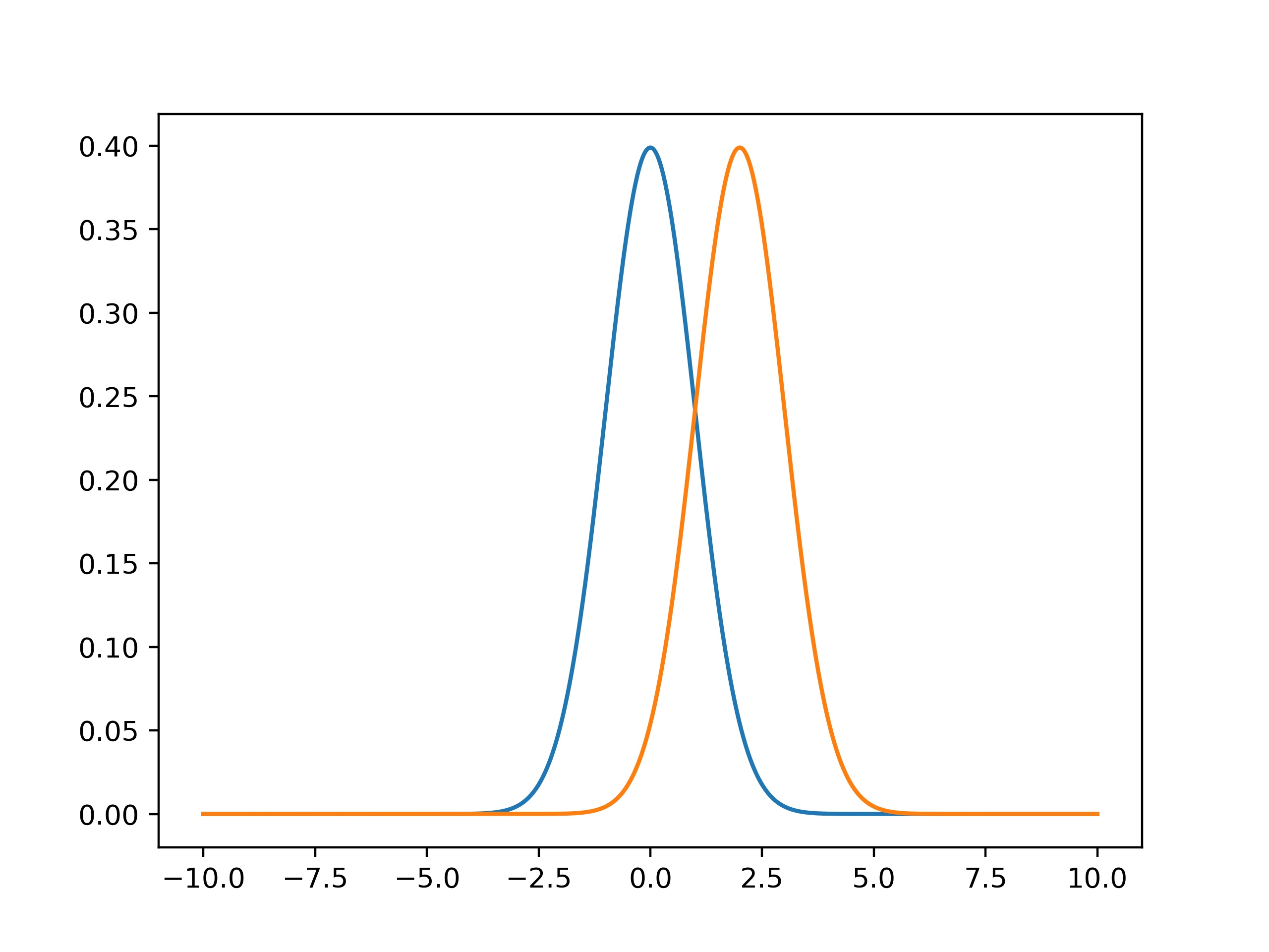
To see whether two values \(P\) and \(Q\) are in agreement, we check whether their difference in values are less than twice their combined uncertainties: \(|P-Q|<2\sqrt{u(P)^2+u(Q)^2} \).

Exercise 6.7
For a certain physics quantity \(E\), Eva has found a value of 14.5\(\pm\)0.2. The literature value of this quantity is 14.9\(\pm\)0.1.

a) Check whether these values are in agreement with each other.

# Answer exercise 6.7a

b) Write a function that makes use of four inputvariables, namely two quantities with their uncertainties. The function should return whether the values are in agreement with each other.

# Answer exercise 6.7b

9.18. Outliers: Chauvenet’s criterium

In a repeated measurement series it is possible that there is an outlier, that deviates largely from the average. You may have made an error while performing the measurement, or it may be caused by random noise. However, it is not allowed to just selectively discard datapoints. Chauvenet’s criterium provides a rule of thumb on when to remove a datapoint, arguing that that a statistical fluctuation is unlikely and there has likely been made a mistake. A datapoint may be removed if \(2N \cdot P_{\text{outlier}} < 0.5\) where \(P_{\text{outlier}} = Erf(x_{\text{outlier}}, \bar x, \sigma)\) when the outlier is below average, and \(P_{\text{outlier}} = 1-Erf(x_{\text{outlier}}, \bar x, \sigma)\) else.

Exercise 6.8
Erin has conducted seven measurements on a capacitor (in \(\mu F\)): 45.7, 53.2, 48.4, 45.1, 51.4, 62.1 and 49.3. The sixth measurement seems suspicious. Use Chauvenet’s criterium to decide whether she should discard that measurement.

# Answer exercise 6.8
C = np.array([45.7, 53.2, 48.4, 45.1, 51.4, 62.1, 49.3])

print('The sixth measurement should (not) be discarded, because ... ')

Exercise 6.8*
In excercise 6.1* you looked at different tree heights. One height stood out.

Would you be allowed to discard the measurment of height 4.5 m? Give a supporting and a counter argument.

9.19. Poisson distribution

Another widely used probability distribution is the Poisson distribution. Many situations that involve counting are described by the poisson distribution, such as radioactive decay or the number of people in a queue.

In a poisson process with parameter \(\lambda\), the probabilty that \(k\) events occur is:

\[\mathbb{P}[X = k] = \frac{\lambda^k}{k!}e^{-\lambda}\]

The mean counts would be \(\lambda\) and the standard deviation \(\sigma = \sqrt{\lambda}\).

Exercise 6.9
In an experiment with a radioactive source, the number of counts in a specific timeinterval is measured 58 times. This resulted in the following distribution of the counts \(N\):

N (counts)	Frequency
1	1
2	0
3	2
4	3
5	6
6	9
7	11
8	8
9	8
10	6
11	2
12	1
13	1

Calculate:

(a) the total number of counts;

(b) the average number of counts \(\mu\);

(c) the standard deviation \(\sigma\).

If the experiment is to be repeated again using 58 measurements

(d) calculate the expected number of measurements with five or less counts.

# Answer exercise 6.9

print('(a) The total number of counts ... ')
print('(b) The average number of counts ... ')
print('(c) The standard deviation is ... ')
print('(d) The expected number of measurements with five or less counts is ... ')

Exercise 6.9*
A shop owner wants to know how many people visit his shop. He installs a device that counts the number of people that enter the shop every minute. In total 1000 measurements were done.

a Import the person_count.dat file.

b Determine the average value as well as the standard deviation.

c Plot the data in a histogram. What kind of distribution do you think the data is best described by, and why? Plot the distribution function on top of the histogram to check.

9.20. Error propagation

Let’s say you have determined a value in an experiment. When you want to use it in an equation, the uncertainty propagates to the new calculated quantity. In general, we use two methods: the functional approach and the calculus approach.

Functional approach:
For a quantity \(Z(A)\) that depends on \(A\) we have:

\[u(Z) = \frac{Z(A+u(A)) - Z(A-u(A))}{2}\]

Calculus approach:
For a quantity \(Z(A)\) that depends on \(A\) we have:

\[u(Z) = \frac{d Z}{d A} u(A)\]

Multiple variables:
For a quantity \(Z(A,B)\) that depends on multiple variables, the uncertainty is calculated by taking the square root of the sum of squared individual uncertainties:

Functional: \(u(Z) = \sqrt{(\frac{Z(A+u(A)) - Z(A-u(A))}{2})^2 + (\frac{Z(B+u(B)) - Z(B-u(B))}{2})^2}\) Calculus: \(u(Z) = \sqrt{(\frac{\partial Z}{\partial A} u(A))^2 + (\frac{\partial Z}{\partial B} u(B))^2}\)

Exercise 6.10
Give the most important steps in your calculations.

The value of a physical quantity \(A\) is determined to be \(A = 9.274 \pm 0.005\). Calculate the value of the physical quantity \(Z\) and its uncertainty \(\alpha_{Z}\) using the calculus approach and the functional approach, when \(Z\) depends on \(A\) as follows:

(a) \(Z = \sqrt{A}\)

(b) \(Z = \exp⁡{(A^{2})}\)

# Answer exercise 6.10
# add your calculations here
# ...
print('(a) Z =  ... ± ... ')
print('(b) Z =  ... ± ... ')

Exercise 6.11
Give the most important steps in your calculations.

Three physical quantities have been determined to be \(A = 12.3 \pm 0.4\), \(B = 5.6 \pm 0.8\) en C = \(89.0 \pm 0.2\). Calculate the value of the physical quantity \(Z\) and its uncertainty \(u(Z)\) using the calculus approach and/or the functional approach, when \(Z\) depends on \(A\), \(B\), and \(C\) as follows:

(a) \(Z = A - B\)

(b) \(Z = \frac{A B }{C}\)

(c) \(Z = \exp{⁡(\frac{A B}{C})}\)

# Answer exercise 6.11
# add your calculations here

print('(a) Z =  ... ± ... ')
print('(b) Z =  ... ± ... ')
print('(c) Z =  ... ± ... ')

Exercise 6.12
You have both seen the functional and the analytical method for calculating the propagation of an error.

Apply both methods on the following functions:

\[Z(x)=\frac{x-1}{x+1}\]

With \(x = 3.2 \pm 0.2\)

\[ Z(x)=e^{x^2} \]

With \( x = 8.745 \pm 0.005\)

# Solution 6.12
# add your calculations here

9.21. Gaussian Fit

In Notebook 5 (section 5.3.5 Residuals) we have already seen that residuals that are the result of noise in the measurements should typically be normally distributed. To verify if the residuals are indeed normally distributed one can make a histogram of these residuals and compare it with the related normal distribution, as will be done in the following exercise.

Exercise 6.13

Interest in ratios of the human body is of all times. A linear relation between height and weight is suspected. In this exercise, we examine this relation.
Attached is a csv file which contains the height (first column) and the weight (second column) of a (male) person.

a Convert the data to metric units as it is now in inches and in lbs.

b Make a scatter plot and investigate whether there is a linear relation.

c Determine the mean and std of both the height and weight.

d Make a histogram for both and overlay a Gaussian to see if the data follows a normal distribution.

#import data
H_W_data = np.genfromtxt('weight-height.csv',delimiter=',',dtype=float,skip_header=1)
height = []
weight = []

#Convert to metric units


#Calculate mean and std


#Linear function to fit


#Curvefit


#Scatter plot
plt.figure(figsize=(12,4))


plt.show()


#Histogram plot

9.21.1. Additional Exercises

Exercise 6.14 Fitting with a measurement error

When measuring there is always a very real possibility of a systematic error. One of these systematic erros can be found in a mass-springsystem. Normally the period of a mass-spring system is given by: \(T = 2\pi \sqrt{\frac{m}{C}}\). Here \(m\) is the mass and \(C\) is the spring constant. However this formula assumes that you have a massless spring, this is not true unfortunately. This means that the mass of the spring is also vibrating, we should thus change the formula to take this into account. This gives the following equation: \(T = 2\pi \sqrt{\frac{m + \Delta m}{C}}\), where \(\Delta m\) is the systematic error.

With the measurements that we have we can find both the spring constant and its uncertainties. The array m is an array with the values for the measured m and the array T is an array with all the measured data for the period. You can disregard the invalid use of significant figures.

a Plot the data

b Find the parameters \(\Delta m\) and \(C\) with its corresponding uncertainties

c Plot the fitted function over the data and examine the residuals

m = np.array([50, 100, 150, 200, 250, 300])
T = np.array([2.47, 3.43, 4.17, 4.80, 5.35, 5.86])

Exercise 6.15 Gravitational force

The gravitational force between two bodies can be described with Newton’s law of universal gravitation: \(F = \frac{Gm_1m_2}{r^2}\), where \(G\) is the gravitational constant, \(m_i\) the masses of the bodies and \(r\) the distance between the bodies.

Suppose that a meteorite of mass \((4.739\pm0.154)\cdot10^8\)kg at a distance of \((2.983\pm0.037)\cdot10^6\)m is moving towards the earth.

Exercise: Determine the attracting force between the meteorite and earth. Use both the functional and the calculus approach to calculate the uncertainty in \(F\) and compare the results. You can use the following values:

• Earth mass: \((5.9722\pm0.0006)\cdot10^{24}\)kg

• Gravitational constant: \((6.67259\pm0.00030)\cdot10^{-11}\)m\(^3\) s\(^{-2}\) kg\(^{-1}\)

#function for gravitational force
def FG(G,m1,m2,r):
    
#values
G = 6.6759e-11
u_G = 0.00030e-11

m1 = 4.739e8
u_m1 = 0.154e8

m2 = 5.9722e24
u_m2 = 0.0006e24

r = 2.983e6
u_r = 0.037e6

#value of gravitatonal force


#Calculus approach


#functional approach

Exercise 6.16 A mass-spring system

A student measures the position of a simple mass-spring system. Unfortunately, he accidently moves his measuring device during the experiment. He is not sure if the device was put back in the right position and wants to know if there is a systematic error in his data. The dataset consists of 400 position measurements (in cm) over the course of 5 seconds. The data is expected to follow a sine function with an amplitude of 4.5 cm and a period of 0.4 s.

a Import the meting_massaveer.dat file.

b Plot the raw data, calculate and plot the residuals, and use it to determine if there is a systematic error. If so, determine the size and time of the shift.

m_C_data = np.genfromtxt('meting_massaveer.dat')
t = np.linspace(0,5,400)

def sine(x):                        #sine function to fit the data
      return 4.5*np.sin(2*np.pi*2.5*x)

#plot of data and sine function

#calculate residuals

#plot of Residuals

9.22. Solutions to Exercises

# Solution 6.1
# Data
V = np.array([25.8, 26.2, 26.0, 26.5, 25.8, 26.1, 25.8, 26.3])

# Edit
Vmean = np.mean(V)
Vstd = np.std(V,ddof=1)
Verr = Vstd/np.sqrt(len(V))

#Print
print('(a) The average is: {} ml' .format(round(Vmean,2)))
print('(b) The standard deviation is: {} ml'.format(round(Vstd,2)))
print('(c) The uncertainty in the mean of the volume: {} ml'.format(round(Verr,2)))
print('(d) The best estimate of the true volume is: {:.2f} \u00B1 {:.2f} ml'.format(Vmean,Verr))

# Solution 6.1*
# add your calculations here

#calculate mean and std 'manually'
Tree_av = np.sum(L)/len(L)
Tree_std = np.sqrt(np.sum((L-Tree_av)**2)/(len(L)-1))

print('The best estimate for the height %.0f +/- %.0f m' %(Tree_av, Tree_std/np.sqrt(len(L))))

#Compare values with numpy functions, if true, nothing happens
assert Tree_av == np.mean(L), 'The results for the mean are different'
assert Tree_std == np.std(L,ddof=1), 'The results for the standard deviation are different'

# Solution 6.2
opg2_1 = 'iii'
opg2_2 = 'vii'
print('The measurements adequately displayed are: {} en {}'.format(opg2_1,opg2_2))

#Solution 6.3
#Data
numbers = np.array([602.20,0.00135,0.0225,1.60219,91.095])

#Print
print('The correct notation of (a) is: {:.1e}'.format(numbers[0]))
print('The correct notation of (b) is: {:.1e}'.format(numbers[1]))
print('The correct notation of (c) is: {:.1e}'.format(numbers[2]))
print('The correct notation of (d) is: {:.1e}'.format(numbers[3]))
print('The correct notation of (e) is: {:.1e}'.format(numbers[4]))

#Solution 6.4
data = np.loadtxt('experimental_results.csv')

N = len(data)
mean_val = np.mean(data)

plt.hist(data,bins=np.linspace(0,2*mean_val,50))
plt.xlabel('Value (-)')
plt.ylabel('Counts (-)')
plt.show()

# Calculation of mean and standard deviation
mean_array = np.zeros(N)
sigma_array = np.zeros(N)

for i in range(N):
    mean_array[i] = np.mean(data[:i+1])
    sigma_array[i] = np.std(data[:i+1], ddof=1)/(i+1)
    
# Plotting
plt.figure()
plt.plot(mean_array)
plt.axhline(mean_val,linestyle='dashed',color='grey')
plt.grid()
plt.xlabel('Data length (-)')
plt.ylabel('Average (-)')
plt.show()

plt.figure()
plt.loglog(sigma_array)
plt.grid()
plt.xlabel('Data length (-)')
plt.ylabel('Uncertainty (-)')
plt.show()

#Solution 6.5

# Input
mu = 502                   # mean
sigma = 14                 # standard deviation

# Values to be measured
x1 = 500
x2 = 530

# Calculation
Pa = norm.cdf(x1,mu,sigma)      # calc: Pa = 0.44320150
Pb = 1 - norm.cdf(x2,mu,sigma)  # calc: Pb = 1 - 0.97724987
aantal = Pb * 1000

#Print
print('(a) P = {:.4f}'.format(Pa))
print('(b) Expected amount = {:.2f}'.format(aantal))

#Solution 6.6

# a. Each series of measurements consists of five repeated measurements.
Measurements = np.array([[4.560,4.470,4.620,4.570,4.570],\
                     [4.570,4.540,4.700,4.510,4.150],\
                     [4.540,4.570,4.550,4.430,4.460],\
                     [4.470,5.130,4.490,5.150,4.530],\
                     [4.400,5.050,4.490,5.080,4.530],\
                     [4.530,5.130,4.560,4.910,4.560]]) #s

# b
# Random error: reaction time, teacher walks in front of the setup
# Systematic error: inertia of lamp in turning off and on (the lamps keeps glowing for a certain amount of time)

# c. The average of the measurement series
Measurements_av = np.array([np.mean(Measurements[0,:]),np.mean(Measurements[1,:]),\
                       np.mean(Measurements[2,:]),np.mean(Measurements[3,:]),\
                       np.mean(Measurements[4,:]),np.mean(Measurements[5,:])])


print('The average times, in s, are: ', np.round(Measurements_av,1))


# Standerd deviation of the measurements series
Measurements_std = np.array([np.std(Measurements[0,:],ddof=1),np.std(Measurements[1,:],ddof=1),\
                         np.std(Measurements[2,:],ddof=1),np.std(Measurements[3,:],ddof=1),\
                         np.std(Measurements[4,:],ddof=1),np.std(Measurements[0,:],ddof=1)])

print('The standard deviation in the times, in s, are: ', np.round(Measurements_std,1))
print('')


# d. Standard deviation in the mean
std_van_gem = np.std(Measurements_av,ddof=1)
print('The standard deviation in the mean is: ', np.round(std_van_gem,1), 's')


# Uncertainty in the measurement series
Measurements_unc = Measurements_std/np.sqrt(5)
print('The uncertainty in each measurement series: ', np.round(Measurements_unc,2), 's')
print('The mean uncertainty: ', np.round(np.mean(Measurements_unc),2), 's')
print()


# e. Final answer
print('The time during which the lamp is on: ', round(np.mean(Measurements),2), '+/-', round(np.std(Measurements,ddof=1)/np.sqrt(30),2),'s')
#Note: We act like the the 6 measurement series are just one big data set

# Solution 6.7

E = 14.5
u_E = 0.2
L = 14.9
u_L = 0.1

if (E-L) > 2*np.sqrt(u_E**2+u_L**2):
    print('No agreement')
else:
    print('The values are in agreement')

#Solution 6.8

#Data
Q = np.array([45.7, 53.2, 48.4, 45.1, 51.4, 62.1, 49.3])
N = len(Q)        # Total number of measurements

#Number to be determined
n = 6             # Number of measurement

#Editing
Qmean = np.mean(Q)
Qstd = np.std(Q,ddof=1)
Qerr = Qstd/np.sqrt(N)
Pout = 1-norm.cdf(Q[n-1],Qmean,Qstd)

#Print
print('The average is: {:.4f} uC'.format(Qmean))
print('The standard deviation is: {:.4f} uC'.format(Qstd))
print('The standard error is: {:.4f} uC'.format(Qerr))
print('Pout = {:.4f}'.format(Pout))
if 2*Pout*N < 0.5:
    print('Measurement {} has to be excluded'.format(n))
else:
    print('Measurement {} cannot be excluded'.format(n))

#Solution 6.8*
print('The 4.5 m may not be a faulty measurement, and can therefore not be discarded.')
print('The 4.5 m deviates from the other tree heights and may be another type or may be planted later.')

#Solution 6.9

#Data
N = np.array([0,1,2,3,4,5,6,7,8,9,10,11,12,13])
f = np.array([0,1,0,2,3,6,9,11,8,8,6,2,1,1])

#Calculations (a)
N_tot = sum(N*f)              # (a) Total number of counts
print('(a) The total number of counts is {:.0f}'.format(Ntot))
print()

#Calculations (b)
N_mean = sum(N*f)/sum(f)        # (b) Average number of counts
print('(b) The average number of counts is {:.2f}'.format(N_mean))
print()

#Calculations (c)
Nstd = np.sqrt(N_mean)              # (c) Standard deviation
Nerr = Nstd / np.sqrt(N_tot)

print('(c) The standard deiation is {:.2f}'.format(Nstd))
print()

#Calculations (d)
P=0
for i in range(6):
    P += N_mean**i*np.exp(-N_mean)/math.factorial(i)
print('(d) The expected number is {:.0f}'.format(P*58))

#Solution 6.9*

persons = np.genfromtxt("person_count.dat") #! aantal_peronen = persons
persons_mean = np.mean(persons)
persons_std = np.std(persons, ddof=1)

print('Average: %.3f \n Standard deviation: %.3f' %(persons_mean,persons_std))

num_bins = int(max(persons)-min(persons))

x = np.linspace(min(persons),max(persons),num_bins+1)
prob = poisson(persons_mean)

f,g,_ = plt.hist(persons,bins=num_bins,density=1)
plt.plot(x+.5,prob.pmf(x),'k.')
plt.xlabel('Number of visitors per minute')
plt.ylabel('Probability')
plt.show()

print('It looks like a Poisson distribution. It concerns a counting experiment, so that makes sense.')

# Solution 6.10

def func2a(a):
    z = np.sqrt(a)
    return z

def calc2a(a,ua):
    uz = np.abs( (1/2) * a**(-1/2) ) * ua
    return uz

def func2b(a):
    z = np.exp(a**2)
    return z

def calc2b(a,ua):
    uz = np.abs( 2 * a * np.exp(a**2) ) * ua
    return uz

a = 1.274
ua = 0.005

za = func2a(a)
uza_func = ( func2a(a+ua)-func2a(a-ua) ) / 2
uza_calc = calc2a(a,ua)
zb = func2b(a)
uzb_func = ( func2b(a+ua)-func2b(a-ua) ) / 2
uzb_calc = calc2b(a,ua)

# The number of significant figures is only given for demonstrative purposes
print('(a) functional: Z = {:.4f} \u00B1 {:.6f}'.format(za,uza_func))
print('      calculus: Z = {:.4f} \u00B1 {:.6f}'.format(za,uza_calc))
print('(b) functional: Z = {:.4f} \u00B1 {:.5f}'.format(zb,uzb_func))
print('      calculus: Z = {:.4f} \u00B1 {:.5f}'.format(zb,uzb_calc))

# Solution 6.11
# add your calculations here

# data
a = 12.3
ua = 0.4

b = 5.6
ub = 0.8

c = 89.0
uc = 0.2

# (a)
za = a - b
uza = np.sqrt( ua**2 + ub**2 )

# (b)
zb = a*b/c
uzb = zb * np.sqrt( (ua/a)**2 + (ub/b)**2 + (uc/c)**2 )

# (c)
zc = np.exp(a*b/c)
dzc_da = (b/c) * np.exp(a*b/c)
dzc_db = (a/c) * np.exp(a*b/c)
dzc_dc = (-a*b/c**2) * np.exp(a*b/c)
uzc = np.sqrt( dzc_da**2 * ua**2 + dzc_db**2 * ub**2 + dzc_dc**2 * uc**2 )

print('(a) Z = {:.1f} \u00B1 {:.1f}  (calculus)'.format(za,uza))
print('(b) Z = {:.1f} \u00B1 {:.1f}  (simplified calculus)'.format(zb,uzb))
print('(c) Z = {:.1f} \u00B1 {:.1f}  (calculus)'.format(zc,uzc))

# Solution 6.12
# add your calculations here
def func1(x):                      #first function
    return (x-1)/(x+1)

def func2(r):                      #second function
    return np.exp(r**2)

def functional(x,sig,f):           #function for the functional method
    return (f(x+sig) - f(x-sig))/2

#first function 
x = 3.2
sig = 0.2
error_functional = functional(x,sig,func1)
error_calculus = sig*((x+1)-(x-1))/(x+1)**2 

print('First function \n\
Value of Z: %.2f \n\
Error with functional approach: %.2f \n\
Error with calculus approach: %.2f \n\
' %(func1(x),error_functional,error_calculus))

#second function
r = 8.745
sig = 0.005
error_functional = functional(r,sig,func2)
error_calculus = sig*2*r*func2(r)  


print('Second function \n\
Value of Z: %.1e \n\
Error with functional approach: %.0e \n\
Error with calculus approach: %.0e \
' %(func2(x),error_functional,error_calculus))

#Solution 6.13
#import data
H_W_data = np.genfromtxt('weight-height.csv',delimiter=',',dtype=float,skip_header=1)
height = []
weight = []

for i in H_W_data:
    height.append(i[0]*2.54)   #convert to cm
    weight.append(i[1]*0.4536) #convert to kg

#Calculate mean and std
height_mean = np.mean(height)
height_std = np.std(height, ddof=1)
weight_mean = np.mean(weight)
weight_std = np.std(weight)

#Linear function to fit
def lin(x,a,b):
    return a*x + b

#Curvefit
val, cov = curve_fit(lin,height,weight)

x = np.linspace(145,205)
y = lin(x,val[0],val[1])

#Scatterplot
plt.figure(figsize=(12,4))
plt.plot(height,weight,'.',label='data')
plt.plot(x,y,label='fit')
plt.xlabel('Height (cm)')
plt.ylabel('Mass (kg)')
plt.xlim(min(x),max(x))
plt.show()

#Histogram plot
N=200
x2 = np.linspace(np.min(height),np.max(height),N)

plt.figure()
x1, y1, _ = plt.hist(height,bins=100)
dist = norm.pdf(x2,height_mean,height_std)
plt.plot(x2,dist*x1.max()/np.max(dist),'r')
plt.xlabel('Height (cm)')
plt.ylabel('Occurence')
plt.show()

#Histogram plot
N=50
x2 = np.linspace(np.min(weight),np.max(weight),N)

plt.figure()
x1, y1, _ = plt.hist(weight,bins=100)
dist = norm.pdf(x2,weight_mean,weight_std)
plt.plot(x2,dist*x1.max()/np.max(dist),'r')
plt.xlabel('Mass (kg)')
plt.ylabel('Occurence')
plt.show()

#Solution 6.14

m = np.array([50,100,150,200,250,300])
T = np.array([2.47,3.43,4.17,4.80,5.35,5.86])


#Define Function to fit
def Per(m,dm,C):
    return 2*np.pi*np.sqrt((m+dm)/C)

#Make figure
fig = plt.figure(figsize=(10,5))
ax = fig.add_subplot(121)
ax.errorbar(m,T,linestyle='none',marker='o')
ax.set_xlabel('m [kg]')
ax.set_ylabel('T [s]')

#Make Fit
vals, uncmat = curve_fit(Per,m,T)

#Make linspace
linm = np.linspace(0.7*np.min(m),1.1*np.max(m),200)

#Plot the fitted line
ax.plot(linm,Per(linm,*vals))

#Set the x-limit
ax.set_xlim(np.min(linm),np.max(linm))

#Find the uncertainties
u_dm, u_C = np.sqrt(np.diag(uncmat))


#Print the values gotten and its uncertainties
print('dm = {:.1f} +/- {:.1f} m'.format(vals[0],u_dm))
print('C = {:.1f} +/- {:.1f} kg m/s^2'.format(vals[1],u_C))

#Make a residual analysis
r = T - Per(m,*popt)

#Plot the risiduals
ax2 = fig.add_subplot(122)
ax2.plot(m,r,linestyle='none',marker='o')
ax2.set_xlabel('m [kg]')
ax2.set_ylabel('R [s]')

#Make it a bit pretier
plt.tight_layout()

#Solution 6.15
#function for gravitational force
def FG(G,m1,m2,r):
    return G * m1 * m2 /(r*r)

#values
G = 6.6759e-11
u_G = 0.00030e-11

m1 = 4.739e8
u_m1 = 0.154e8

m2 = 5.9722e24
u_m2 = 0.0006e24

r = 2.983e6
u_r = 0.037e6

#value of gravitatonal force
F_m = FG(G,m1,m2,r)

#calculus appraoch
r2 = r**2
u_F2 = (m1*m2/r2*u_G)**2 + (G*m2/r2*u_m1)**2 + (G*m1/r2*u_m2)**2 + (-2*G*m1*m2/(r2*r)*u_r)**2
u_F_calc = np.sqrt(u_F2)

#Func
U_F2 = ((FG(G+u_G,m1,m2,r)-FG(G-u_G,m1,m2,r))/2)**2 + ((FG(G,m1+u_m1,m2,r)-FG(G,m1-u_m1,m2,r))/2)**2 + ((FG(G,m1,m2+u_m2,r)-FG(G,m1,m2-u_m2,r))/2)**2 + ((FG(G,m1,m2,r+u_r)-FG(G,m1,m2,r-u_r))/2)**2
u_F_func = np.sqrt(U_F2)

print("F = %.2f +/- %.2f 10^10 N \n" %(F_m/1e10,u_F_func/1e10))

diff = np.abs(u_F_calc-u_F_func)

#onzekerheid in veel decimale cijfers om verschil te tonen
print("Uncertainties \n\
Caluculus approach: %f 10^8 N \n\
Functional approach: %f 10^8 N \n\
Difference: %f 10^8 N" %(u_F_calc/1e8,u_F_func/1e8,diff/1e8))

#Solution 6.16
data = np.genfromtxt('meting_massaveer.dat')
t = np.linspace(0,5,400)

def sine(x):                        #sine function to fit the data
      return 4.5*np.sin(x*5*np.pi)

#plot of data and sine function
plt.figure(figsize=(12,4))
plt.title('Data')
plt.plot(t,data, '.', label='data')
plt.plot(t,sine(t), label='$4.5\sin(5\pi x$)')
plt.xlim(min(t),max(t))
plt.ylabel('Position (cm)')
plt.xlabel('Time (s)')
plt.legend()
plt.show()

R = data - sine(t)  #Residuals

#plot of Residuals
plt.figure(figsize=(12,4))
plt.title('Residuals')
plt.plot(t,R)
plt.ylabel('Position (cm)')
plt.xlabel('Time (s)')
plt.show()

plt.hist(R[:100])
plt.show()

# Solution (PRE/POST EXERCISE)
I = np.array([3034,1494,756.1,384.9,199.5,100.6,39.93,20.11,10.23,5.00,2.556,1.269,0.601,0.295,0.137,0.067])*1e-6
a_I = np.array([4,2,0.8,0.4,0.3,0.2,0.05,0.03,0.02,0.01,0.008,0.007,0.007,0.006,0.006,0.006])*1e-6
V = np.array([670,636,604,572,541,505,465,432,400,365,331,296,257,221,181,145])*1e-3
a_V = np.array([4,4,4,4,4,4,3,3,3,3,3,2,2,2,2,2])*1e-3

def current(V,a,b):
    return a*(np.exp(b*V)-1)

popt, pcov = curve_fit(current,V,I)
x = np.linspace(0.1,0.7)
y = current(x,popt[0],popt[1])

plt.figure(figsize=(8,4))
plt.errorbar(V,I,xerr=a_V,yerr=a_I,linestyle='none',marker= '.',label='data')
plt.plot(x,y,label='fit')
plt.yscale('log')
plt.xlabel('Voltage (V)')
plt.ylabel('Current (A)')
#plt.legend()
plt.xlim(0.1,0.7)
plt.show()
print('The model is in good agreement with the measurements, it is therefore a valid model.')


# agreement analysis
print('a = %.3g +/- %.1g' %(popt[0], np.sqrt(pcov[0,0])))

a_2 = 2.0e-9
u_a_2 = 5e-10

if 2*np.sqrt(u_a_2**2 + pcov[0,0]) > np.abs(a_2 - popt[0]):
    print('The value of $a$ found in the experiment is in agreement with the value from theory,')
else:
    print('The value of $a$ found in the experiment does not agree with the value from theory,')