02 Skipping Rope

Aim¶

To show that in a skipping rope an electric voltage is induced. (The strength of the Earth’s magnetic field can be determined.)

Subjects¶

• 5K10 (Induced Currents and Forces)

Diagram¶

Equipment¶

• Compass needle.

• Skipping rope; $10 \mathrm{~m}$ of a heavy flexible insulated copper wire.

• Overheadsheet with drawing of skipping rope catenary, to determine area.

• Operational amplifier, amplification factor $=1000$.

• Oscilloscope.

• Data-acquisition system .

• Projector to project monitor image.

Presentation¶

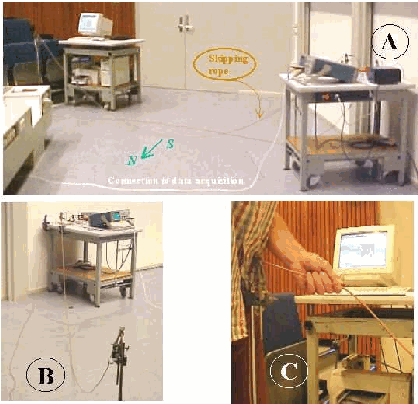
The compass needle is placed on the overheadprojector to indicate the North-South direction in the lecturehall.

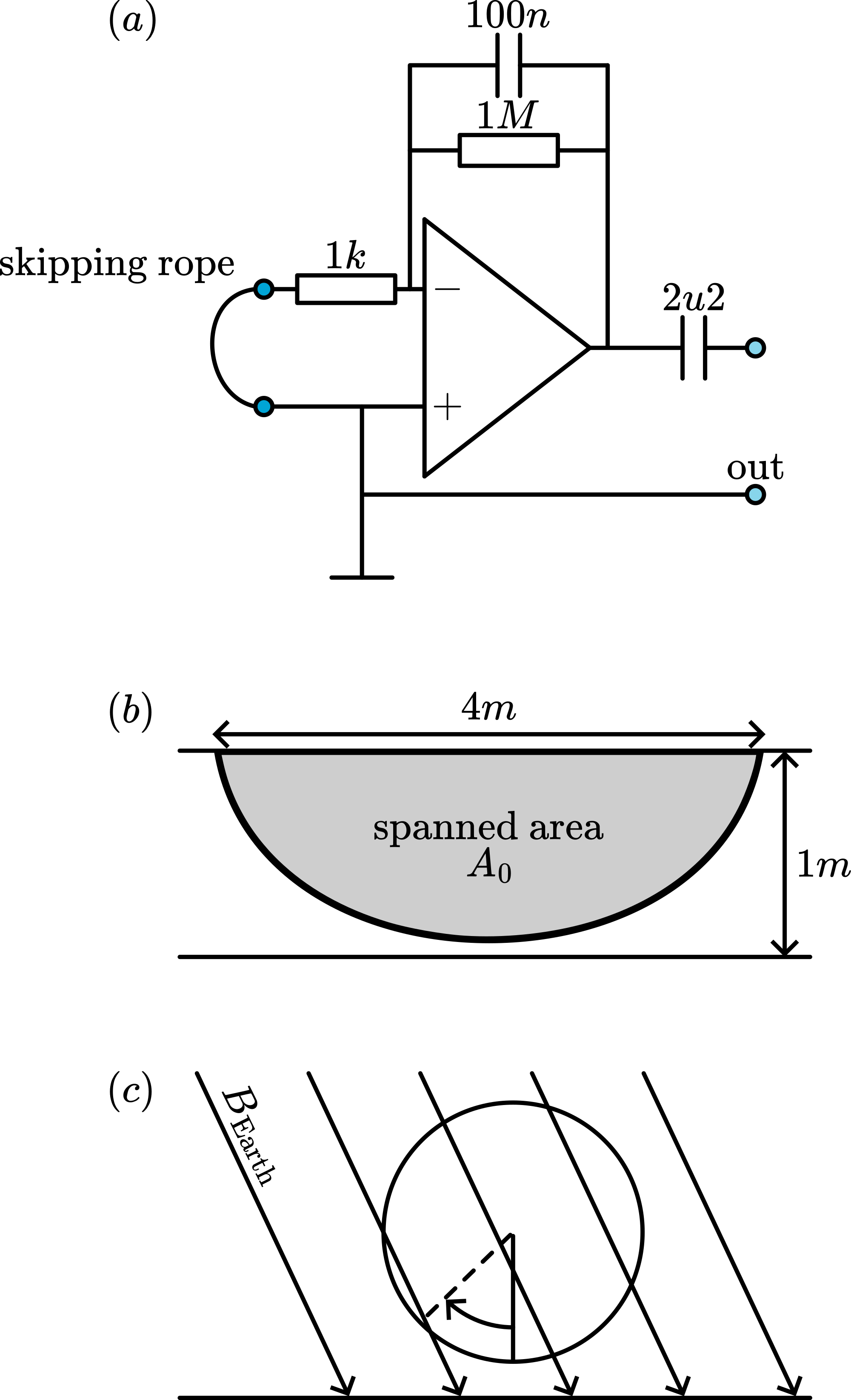
The demonstration is set up as shown in Diagram, and positioned so that the axis of rotation of the skipping rope is perpendicular to the indicated $\mathrm{N}$-S direction (see Diagram A). The skipping rope is connected to the operational amplifier circuit (see Figure 2A). The output of the amplifier is connected to the oscilloscope, having a slowly moving time-base (.1sec/DIV).

The skipping rope is set in rotation (see Diagram C) and the moving spot on the oscilloscope screen is seen to move up and down, showing positive - and negative induced voltages. When the skipping rope is speeded up the amplitude of the induced voltage increases.

In order to observe the induced voltage more in detail, the output is also connected to the interface of the data-acquisition system. A voltage-time graph is displayed to the students and they observe the registration of the (1000 times amplified) induced voltage while the skipping rope is making about 15 full turns, some slow, some fast (see Figure 3). Clearly the sinusoidal shape of the induced voltage can be observed.

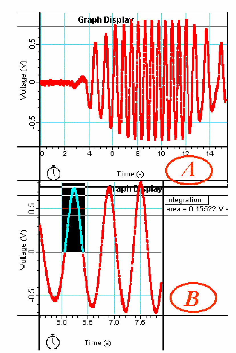
Finally, a part of the graph with a full cycle is selected and by means of the graph features in the statistics software the integration of a selected one half of a sine is determined (see Figure 3B). We read $0.155 \mathrm{~V}$. Applying Faraday’s induction law and estimating the area of the skipping rope (use the overheadsheet), we find for the Earth’s magnetic field $B_{0}=28 U T$ (see Explanation). This is good enough (good enough for a demonstration) when compared with values given in literature.

Explanation¶

The induced voltage ( $E$ ) is given by Faraday’s induction law as $E(t)=B_{0} \frac{d A}{d t} . B_{0}$ is the magnetic flux density; $A$ is the area spanned by the skipping rope and its rotational axis. The plane of the skipping rope changes as $A=A_{0} \cos \omega t$ (see Figure 2C), so $\frac{d A}{d t}=-A_{0} \sin \omega t$, and $E(t)=B_{0} A_{0} \omega$ sin $\omega t$ : the induced voltage $(E)$ changes sinusoidally as the registered graph shows convincingly.

An interesting quantity is $\int E(t) d t$ (voltage surge, or voltage impulse, in units [Vs]). We will use this quantity to determine the Earth’s magnetic field.

From Faraday’s induction law: $E(t) d t=-B_{0} d A$ and $\frac{d A}{d t}=-A_{0} \omega \sin \omega t$, we get:

$\int E(t) d t=-B_{0} A_{0} \omega \int \sin \omega t d t$. When we look at one half of a full cycle, we have:

$\int E(t) d t=-B_{0} A_{0} \cos (\omega t)_{0}^{\pi}=2 B_{0} A_{0}$. From Figure 3B we read $\int E(t) d t$ equals

$0,155 \mathrm{~V}$. Figure 2B is used to estimate the area $A_{o}$ of the catenary of the suspended skipping rope. With the dimensions given, we estimate a little less than $3 \mathrm{~m}^{2}$, so let us say $2.8 \mathrm{~m}^{2}$. With these numbers we find for the Earth’s magnetic field: $B_{0}=28 U T$.

Remarks¶

• In the operational amplifier circuit the $100 \mathrm{nF}$ capacitor is needed to reduce the noise of the mains. The $2,2 \mathrm{uF}$ capacitor is applied to block the dc-offset that is usually present at the output of such amplifiers.

• The table with amplifier and oscilloscope has to stand firmly on the ground (see DiagramB), because rotating the rope gives forceful jerks to that table.

• The registered induced voltage is not really symmetrical (see Figure 3) this is due to the way of turning such a skipping rope: at each cycle you give a kind of jerk when swinging the rope upwards, so in its cycle the angular speed is not really constant.

• During the first run, when registering the voltage-time graph, we make the statistics software indicate the mean y-value (voltage). In that way it is seen that the first and last not so beautiful movement of the skipping rope has not really a significant influence on our further measurements.

Sources¶

• Mansfield, M and O’Sullivan, C., Understanding physics, pag. 514-515 and 524-525

• The Physics Teacher, pag. Vol.41, nr.5, pp295-297