# Matplotlib compatibility patch for Pyodide
import matplotlib
if not hasattr(matplotlib.RcParams, "_get"):
    matplotlib.RcParams._get = dict.get
Exercises#
Repeated readings and measurement uncertainty#
Exercise 6.1
The results of eight titrated volumes (in ml) are: 25.8, 26.2, 26.0, 26.5, 25.8, 26.1, 25.8 and 26.3.
Calculate:
(i) the average,
(ii) the standard deviation,
(iii) the uncertainty in the mean of the volume,
(iv) present the best estimate of the true volume with its associated uncertainty.
# Answer exercise 6.1:
V = np.array([25.8, 26.2, 26.0, 26.5, 25.8, 26.1, 25.8, 26.3])
#Your code


print('The average is: ')

print('The standard deviation is: ')

print('The uncertainty in the mean of the volume: ')

print('The best estimate of the true volume is: ' )
Exercise 6.1*
You probably know the np.mean and the np.std commands. However you can also do them yourself using the definitions:
Use these on the following dataset and see if you get the same results as the np.mean and the np.std commands.
Data
Tree Number |
Total Height (m) |
|---|---|
1 |
14.02 |
2 |
14.15 |
3 |
15.27 |
4 |
11.81 |
5 |
14.22 |
6 |
20.52 |
7 |
18.2 |
8 |
16.92 |
9 |
16.28 |
10 |
20.8 |
11 |
4.5 |
Models of knot and stem development in black spruce trees indicate a shift in allocation priority to branches when growth is limited. Available from: https://www.researchgate.net/figure/Characteristics-of-the-10-sample-trees-in-the-dataset_tbl1_274717928 [accessed 24 Jul, 2020]
a Calculate in two different ways the mean value and the standard deviation.
b If you notice a difference between the np.std function and the manual function I would encourage you to look at the documentation of the np.std function Here.
c How would you as a physicist write down the result?
L = np.array([14.02,14.15,15.27,11.81,14.22,20.52,18.2,16.92,16.28,20.8,4.5])
#your code
Exercise 6.2
Below are eight resistor measurements, each based on ten repeated readings. However, only two measurements are adequately displayed.
Which ones?
(i) \((99.8 \pm 0.270) \cdot 10^3 \,\Omega\)
(ii) \((100 \pm 0.3) \cdot 10^3 \,\Omega\)
(iii) \((100.0 \pm 0.3) \cdot 10^3 \,\Omega\)
(iv) $(100.1 \pm 0.3) \cdot 10^3 $
(v) \(99.4 \cdot 10^3 \pm 36.0 \cdot 10^2 \,\Omega\)
(vi) \(101.5 \cdot 10^3 \pm 0.3 \cdot 10^1 \,\Omega\)
(vii) \((99.8 \pm 0.3) \cdot 10^3 \,\Omega\)
(viii) \(95.2 \cdot 10^3 \pm 273 \,\Omega\)
# Answer exercise 6.2
print('The measurements adequately displayed are: ')
Exercise 6.3
Round the following numbers displaying two figures and use scientific notation.
(i) 602.20
(ii) 0.00135
(iii) 0.0225
(iv) 1.60219
(v) 91.095
# Answer exercise 6.3
print('The correct notation of (i) is: ')
print('The correct notation of (ii) is: ')
print('The correct notation of (iii) is: ')
print('The correct notation of (iv) is: ')
print('The correct notation of (v) is: ')
So, let us look at what happens when we repeat our measurements. How does this change our best estimate of the true value, and how does repeating measurements decrease the measurement uncertainty?
Exercise 6.4
During an experiment, an automated reading of a certain quantity is carried out. The data is stored in the file ‘experimental_results.csv’.
a Load the data.
b Calculate the average value and the standard deviation. Plot as well the histogram of the readings.
# your code for 6.4 a and b.
We expect that the average value converges to a certain value (the true value) when we increase the number of repeated readings.
c Plot the average value as function of the number of repeated readings. Thereto, make an array in which the average value as function of the number of repeated readings is stored.
We also expect that the uncertainty in the average value decreases with an increasing number of repeated readings.
d Plot the uncertainty in the average value as function of the number of repeated readings. Use a log-log scale.
# your code for 6.4 c and d.
Normal distribution#
A measurement \(M\) can be interpreted as the physical quantities’ true value \(G\) and some unwanted noise \(s\): \(M = G + s\). In many cases, this noise is normally distributed. For a normal distribution with mean \(\mu\), and standard deviation \(\sigma\), the probability density function is given by
In general, a probability density \(p(x)\) is a function that has the property that the probabilty that a random variable \(X\) has a value smaller than \(x\) is given by:
The normal distribution is sometimes called a Gaussian distribution, and its density function is sometimes called a Bell curve. Unfortunately, it is not possible to analytically solve the integral of the density of the normal distribution. Luckily, good numerical approximations of this integral, that is also called the errorfunction \(Erf(x,\mu, \sigma)\), exist. In python you can use scipy.stats.norm.pdf for the probabilty density function, and scipy.stats.norm.cdf for the error function. [https://docs.scipy.org/doc/scipy/reference/generated/scipy.stats.norm.html].
Exercise 6.5
Bags of rice with indicated weight of 500 g are sold. In practice, this weight is normally distributed with an average weight of 502 g and a standard deviation of 14 g.
(a) What is the chance that a bag of rice weights less than 500 g?
(b) If we would buy 1000 bags of rice, how many can be expected to weigh at least 530 g? Use the error function, Erf(\(x\); \(\bar{x}\), \(\sigma\)) or scipy.stats.norm.cdf to compute this expectation.
# Answer exercise 6.5

print('(a)  P = ... ')
print('(b)  number = ...')
from scipy.stats import norm

x = np.linspace(-10,10,100)
plt.plot(x, norm.pdf(x, 0,1))
plt.plot(x, norm.cdf(x,0,1))
plt.show()
Exercise 6.6
In the movieclip below you see a blinking LED. Here we investigate how long the LED is ON.
(a) Take 15 (3 sets of 5) repeated readings of the time that the LED is ON. Note these measurements in the array below. Also ask the dataset of someone else so you have 6x5 repeated readings.
(b) Provide a reason for a potential systematic error and two reasons for potential random errors.
(c) For each of set of five repeated readings calculate the average time \(\mu(t)\) the LED is on and the associated standard deviation \(\sigma(t)\) and the uncertainty \(u(t)\).
The average time found is probably not the same each time. We can calculate the standard deviation of the mean of each set of five readings.
(d) Calculate the standard deviation of the mean.
(e) Compare the standard deviation of the mean with the mean of the uncertainty of the 6 sets. Are these two values comparable?
(f) Provide the best estimate of the time \(\mu(t) \pm u(t)\) that the LED is on. Use the scientific conventions for presenting your result.
# Answer exercise 6.6
Measurements = np.array([[,,,,],\
                     [,,,,],\
                     [,,,,],\
                     [,,,,],\
                     [,,,,],\
                     [,,,,]]) #s


Measurements_av = np.array([np.mean(),\
                       np.mean(),\
                       np.mean()])
Agreement analysis#
If we have found a certain value and want to compare it with a known value, when do these values agree with each other? Certainly this depends on the average value found. But in the two figures below, we can also see that this depends on how (un)certain our determined values are. The first values might be in agreement with each other, as their pdf’s overlap. But the second values certainly are not.
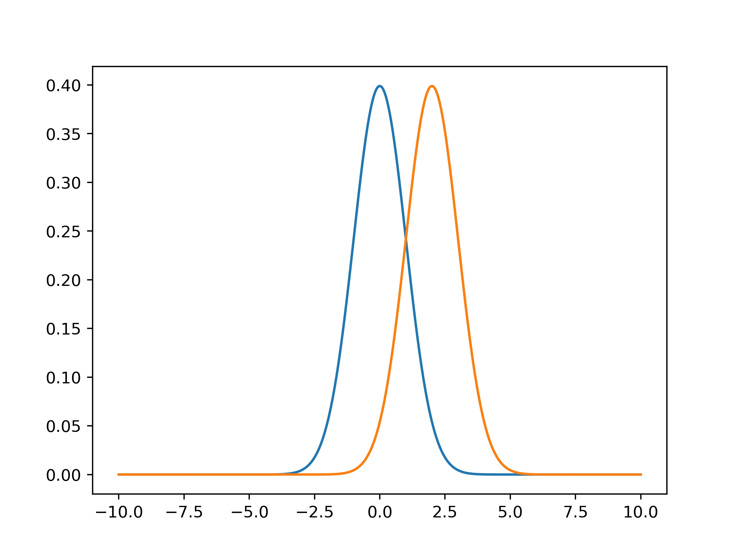
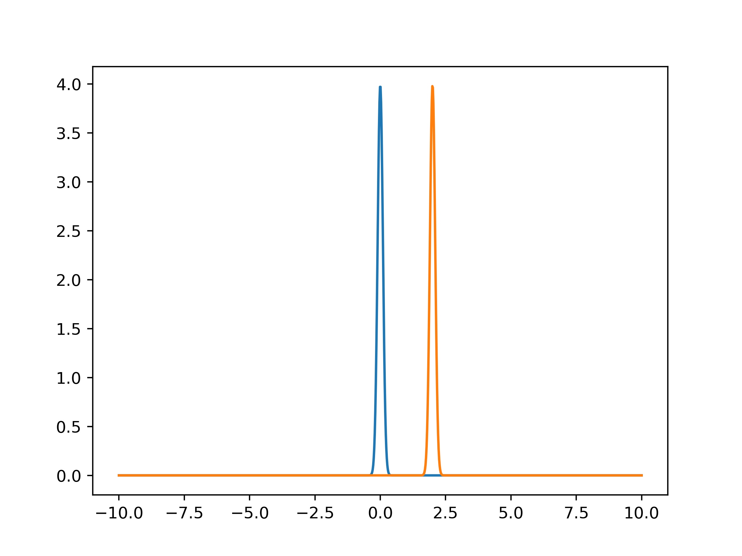
To see whether two values \(P\) and \(Q\) are in agreement, we check whether their difference in values are less than twice their combined uncertainties: \(|P-Q|<2\sqrt{u(P)^2+u(Q)^2} \).
Exercise 6.7
For a certain physics quantity \(E\), Eva has found a value of 14.5\(\pm\)0.2. The literature value of this quantity is 14.9\(\pm\)0.1.
a) Check whether these values are in agreement with each other.
# Answer exercise 6.7a
b) Write a function that makes use of four inputvariables, namely two quantities with their uncertainties. The function should return whether the values are in agreement with each other.
# Answer exercise 6.7b
Outliers: Chauvenet’s criterium#
In a repeated measurement series it is possible that there is an outlier, that deviates largely from the average. You may have made an error while performing the measurement, or it may be caused by random noise. However, it is not allowed to just selectively discard datapoints. Chauvenet’s criterium provides a rule of thumb on when to remove a datapoint, arguing that that a statistical fluctuation is unlikely and there has likely been made a mistake. A datapoint may be removed if \(2N \cdot P_{\text{outlier}} < 0.5\) where \(P_{\text{outlier}} = Erf(x_{\text{outlier}}, \bar x, \sigma)\) when the outlier is below average, and \(P_{\text{outlier}} = 1-Erf(x_{\text{outlier}}, \bar x, \sigma)\) else.
Exercise 6.8
Erin has conducted seven measurements on a capacitor (in \(\mu F\)): 45.7, 53.2, 48.4, 45.1, 51.4, 62.1 and 49.3. The sixth measurement seems suspicious. Use Chauvenet’s criterium to decide whether she should discard that measurement.
# Answer exercise 6.8
C = np.array([45.7, 53.2, 48.4, 45.1, 51.4, 62.1, 49.3])

print('The sixth measurement should (not) be discarded, because ... ')
Exercise 6.8*
In excercise 6.1* you looked at different tree heights. One height stood out.
Would you be allowed to discard the measurment of height 4.5 m? Give a supporting and a counter argument.
Poisson distribution#
Another widely used probability distribution is the Poisson distribution. Many situations that involve counting are described by the poisson distribution, such as radioactive decay or the number of people in a queue.
In a poisson process with parameter \(\lambda\), the probabilty that \(k\) events occur is:
The mean counts would be \(\lambda\) and the standard deviation \(\sigma = \sqrt{\lambda}\).
Exercise 6.9
In an experiment with a radioactive source, the number of counts in a specific timeinterval is measured 58 times. This resulted in the following distribution of the counts \(N\):
N (counts) |
Frequency |
|---|---|
1 |
1 |
2 |
0 |
3 |
2 |
4 |
3 |
5 |
6 |
6 |
9 |
7 |
11 |
8 |
8 |
9 |
8 |
10 |
6 |
11 |
2 |
12 |
1 |
13 |
1 |
Calculate:
(a) the total number of counts;
(b) the average number of counts \(\mu\);
(c) the standard deviation \(\sigma\).
If the experiment is to be repeated again using 58 measurements
(d) calculate the expected number of measurements with five or less counts.
# Answer exercise 6.9

print('(a) The total number of counts ... ')
print('(b) The average number of counts ... ')
print('(c) The standard deviation is ... ')
print('(d) The expected number of measurements with five or less counts is ... ')
Exercise 6.9*
A shop owner wants to know how many people visit his shop. He installs a device that counts the number of people that enter the shop every minute. In total 1000 measurements were done.
a Import the person_count.dat file.
b Determine the average value as well as the standard deviation.
c Plot the data in a histogram. What kind of distribution do you think the data is best described by, and why? Plot the distribution function on top of the histogram to check.
Error propagation #
Let’s say you have determined a value in an experiment. When you want to use it in an equation, the uncertainty propagates to the new calculated quantity. In general, we use two methods: the functional approach and the calculus approach.
Functional approach:
For a quantity \(Z(A)\) that depends on \(A\) we have:
Calculus approach:
For a quantity \(Z(A)\) that depends on \(A\) we have:
Multiple variables:
For a quantity \(Z(A,B)\) that depends on multiple variables, the uncertainty is calculated by taking the square root of the sum of squared individual uncertainties:
Functional: \(u(Z) = \sqrt{(\frac{Z(A+u(A)) - Z(A-u(A))}{2})^2 + (\frac{Z(B+u(B)) - Z(B-u(B))}{2})^2}\) Calculus: \(u(Z) = \sqrt{(\frac{\partial Z}{\partial A} u(A))^2 + (\frac{\partial Z}{\partial B} u(B))^2}\)
Exercise 6.10
Give the most important steps in your calculations.
The value of a physical quantity \(A\) is determined to be \(A = 9.274 \pm 0.005\). Calculate the value of the physical quantity \(Z\) and its uncertainty \(u(Z)\) using the calculus approach and the functional approach, when \(Z\) depends on \(A\) as follows:
(a) \(Z = \sqrt{A}\)
(b) \(Z = \exp{(A^{2})}\)
# Answer exercise 6.10
# add your calculations here
# ...
print('(a) Z =  ... ± ... ')
print('(b) Z =  ... ± ... ')
Exercise 6.11
Give the most important steps in your calculations.
Three physical quantities have been determined to be \(A = 12.3 \pm 0.4\), \(B = 5.6 \pm 0.8\) en C = \(89.0 \pm 0.2\). Calculate the value of the physical quantity \(Z\) and its uncertainty \(u(Z)\) using the calculus approach and/or the functional approach, when \(Z\) depends on \(A\), \(B\), and \(C\) as follows:
(a) \(Z = A - B\)
(b) \(Z = \frac{A B }{C}\)
(c) \(Z = \exp{(\frac{A B}{C})}\)
# Answer exercise 6.11
# add your calculations here

print('(a) Z =  ... ± ... ')
print('(b) Z =  ... ± ... ')
print('(c) Z =  ... ± ... ')
Exercise 6.12
You have both seen the functional and the analytical method for calculating the propagation of an error.
Apply both methods on the following functions:
With \(x = 3.2 \pm 0.2\)
With \( x = 8.745 \pm 0.005\)
# Solution 6.12
# add your calculations here
Gaussian Fit #
In Notebook 5 (section 5.3.5 Residuals) we have already seen that residuals that are the result of noise in the measurements should typically be normally distributed. To verify if the residuals are indeed normally distributed one can make a histogram of these residuals and compare it with the related normal distribution, as will be done in the following exercise.
Exercise 6.13
Interest in ratios of the human body is of all times. A linear relation between height and weight is suspected. In this exercise, we examine this relation.
Attached is a csv file which contains the height (first column) and the weight (second column) of a (male) person.
a Convert the data to metric units as it is now in inches and in lbs.
b Make a scatter plot and investigate whether there is a linear relation.
c Determine the mean and std of both the height and weight.
d Make a histogram for both and overlay a Gaussian to see if the data follows a normal distribution.
#import data
H_W_data = np.genfromtxt('weight-height.csv',delimiter=',',dtype=float,skip_header=1)
height = []
weight = []

#Convert to metric units


#Calculate mean and std


#Linear function to fit


#Curvefit


#Scatter plot
plt.figure(figsize=(12,4))


plt.show()


#Histogram plot
Additional Exercises#
Exercise 6.14 Fitting with a measurement error
When measuring there is always a very real possibility of a systematic error. One of these systematic erros can be found in a mass-springsystem. Normally the period of a mass-spring system is given by: \(T = 2\pi \sqrt{\frac{m}{C}}\). Here \(m\) is the mass and \(C\) is the spring constant. However this formula assumes that you have a massless spring, this is not true unfortunately. This means that the mass of the spring is also vibrating, we should thus change the formula to take this into account. This gives the following equation: \(T = 2\pi \sqrt{\frac{m + \Delta m}{C}}\), where \(\Delta m\) is the systematic error.
With the measurements that we have we can find both the spring constant and its uncertainties. The array m is an array with the values for the measured m and the array T is an array with all the measured data for the period. You can disregard the invalid use of significant figures.
a Plot the data
b Find the parameters \(\Delta m\) and \(C\) with its corresponding uncertainties
c Plot the fitted function over the data and examine the residuals
m = np.array([50, 100, 150, 200, 250, 300])
T = np.array([2.47, 3.43, 4.17, 4.80, 5.35, 5.86])
Exercise 6.15 Gravitational force
The gravitational force between two bodies can be described with Newton’s law of universal gravitation: \(F = \frac{Gm_1m_2}{r^2}\), where \(G\) is the gravitational constant, \(m_i\) the masses of the bodies and \(r\) the distance between the bodies.
Suppose that a meteorite of mass \((4.739\pm0.154)\cdot10^8\)kg at a distance of \((2.983\pm0.037)\cdot10^6\)m is moving towards the earth.
Exercise: Determine the attracting force between the meteorite and earth. Use both the functional and the calculus approach to calculate the uncertainty in \(F\) and compare the results. You can use the following values:
Earth mass: \((5.9722\pm0.0006)\cdot10^{24}\)kg
Gravitational constant: \((6.67259\pm0.00030)\cdot10^{-11}\)m\(^3\) s\(^{-2}\) kg\(^{-1}\)
#function for gravitational force
def FG(G,m1,m2,r):

#values
G = 6.6759e-11
u_G = 0.00030e-11

m1 = 4.739e8
u_m1 = 0.154e8

m2 = 5.9722e24
u_m2 = 0.0006e24

r = 2.983e6
u_r = 0.037e6

#value of gravitatonal force


#Calculus approach


#functional approach
Exercise 6.16 A mass-spring system
A student measures the position of a simple mass-spring system. Unfortunately, he accidently moves his measuring device during the experiment. He is not sure if the device was put back in the right position and wants to know if there is a systematic error in his data. The dataset consists of 400 position measurements (in cm) over the course of 5 seconds. The data is expected to follow a sine function with an amplitude of 4.5 cm and a period of 0.4 s.
a Import the meting_massaveer.dat file.
b Plot the raw data, calculate and plot the residuals, and use it to determine if there is a systematic error. If so, determine the size and time of the shift.
m_C_data = np.genfromtxt('meting_massaveer.dat')
t = np.linspace(0,5,400)

def sine(x):                        #sine function to fit the data
      return 4.5*np.sin(2*np.pi*2.5*x)

#plot of data and sine function

#calculate residuals

#plot of Residuals