# Matplotlib compatibility patch for Pyodide
import matplotlib
if not hasattr(matplotlib.RcParams, "_get"):
    matplotlib.RcParams._get = dict.get
Measurements and their uncertainty#
Pre/Post-test#
This test is for testing your current skills in Python. You can use it in two ways:
pre-test: to test your skills beforehand. If you are already proficient in Python, and can do this test within approximately 15 minutes, you can scan through the notebook rather than carefully reading each sentence.
post-test: test your skills after Notebook 6. Check whether you learned enough.
Diode
In an experiment, 10 measurements were taken of the voltage over and current through a Si-diode. The results are displayed in the following table, together with their uncertainties:
I (μA) |
\(u(I)\) (μA) |
V (mV) |
\(u(V)\) (mV) |
|---|---|---|---|
3034 |
4 |
670 |
4 |
1494 |
2 |
636 |
4 |
756.1 |
0.8 |
604 |
4 |
384.9 |
0.4 |
572 |
4 |
199.5 |
0.3 |
541 |
4 |
100.6 |
0.2 |
505 |
4 |
39.93 |
0.05 |
465 |
3 |
20.11 |
0.03 |
432 |
3 |
10.23 |
0.02 |
400 |
3 |
5.00 |
0.01 |
365 |
3 |
2.556 |
0.008 |
331 |
3 |
1.269 |
0.007 |
296 |
2 |
0.601 |
0.007 |
257 |
2 |
0.295 |
0.006 |
221 |
2 |
0.137 |
0.006 |
181 |
2 |
0.067 |
0.006 |
145 |
2 |
The diode is expected to behave according to the following relation: \(I = a(e^{bV}-1)\), where \(a\) and \(b\) are unknown constants.
Exercise: Use the curve_fit function to determine whether this is a valid model to describe the dataset. Is the value found for parameter \(a\) in agreement with the value found in another experiment \(a_{2} = 2.0 \pm 0.5 \mathrm{nA}\)?
Hint: use a logscale on the y-axis
import numpy as np
import matplotlib.pyplot as plt
from scipy.optimize import curve_fit

I = np.array([3034,1494,756.1,384.9,199.5,100.6,39.93,20.11,10.23,5.00,2.556,1.269,0.601,0.295,0.137,0.067])*1e-6
a_I = np.array([4,2,0.8,0.4,0.3,0.2,0.05,0.03,0.02,0.01,0.008,0.007,0.007,0.006,0.006,0.006])*1e-6
V = np.array([670,636,604,572,541,505,465,432,400,365,331,296,257,221,181,145])*1e-3
a_V = np.array([4,4,4,4,4,4,3,3,3,3,3,2,2,2,2,2])*1e-3
Learning objectives#
Now that we’ve learned the basics of Python, it’s time to apply it to explore features and understand the nature of physical measurements.
In this notebook, we will introduce you to measurements, variance in repeated measurements, and measurement uncertainties. When performing calculations with values that include uncertainties, the results also carry uncertainties — but how do we calculate them? Moreover, we often do not work with a single set of repeated measurements but with datasets containing several mean values of repeated measurements. How do we properly analyze such data?
For each topic, a summary is given. What is new, compared to the previous notebooks, is that we have * assignments. These are not mandatory, but can be made to help you improve your knowledge of Python and data-analysis.
Now that we know how to do some basic Python, it is time to use it to understand features of physical measurements. It is very useful to study the chapter in the online manual as well!
After completing this notebook, you are able to:
calculate the mean, standard deviation and uncertainty of a dataset
report findings using the scientific conventions
understand and use Gaussian and Poisson distribution
identify outliers
carry out an agreement analysis
calculate how uncertainties propagate when calculations are performed
Introduction#
In physics experiments, you try to determine relationships or certain values as accurately as possible. What “as accurately as possible” actually means remains unclear for now. What should already be clear is that we can almost never determine such values directly. Instead, we conduct experiments to collect data, which we then use to determine the relationship and establish its parameters as accurately as possible.
However, it is never possible to determine the exact value(s) of those parameters. Each new measurement will show small fluctuations, especially when measuring with high precision. Over time, we have been able to improve our experiments and take more measurements in less time. This means that, over the course of history, constants such as Planck’s constant have been determined with increasing accuracy and that the value has varied over the years.
The consequence of never being able to determine a value exactly is that any result based on it will also carry uncertainty. It will always be uncertain what the exact value actually is. In this chapter, you will learn how the uncertainty in a measured value affects the final result (you already know the basics, significant figures and associated calculation rules), and how to minimize that uncertainty.
Note
The terms measurement error and measurement uncertainty are often used interchangeably. In many cases, measurement uncertainty would be a more accurate description of the situation. A measurement error implies that you are doing something truly wrong, without being able to do anything about it. The error arises inherently from the use of an instrument, from the measurement itself. In that case, it would be more accurate to talk about uncertainty. Although we try to make a careful distinction here, in general language use the two terms are often unintentionally interchanged.
Goal#
A complete data analysis will often consist of the following three phases:
determining the reliability of individual measurements and the dataset as a whole;
finding and determining the pattern in the data, including determining the variables with their associated uncertainties;
an optimal data (re)presentation to convince of phases 1 & 2.
The aim of this part of the physics practical is to develop a deeper understanding of the above phases and to learn how to apply the associated techniques.
Quantities, units, dimension-analysis and constants#
In physics, we measure physical quantities. We distinguish between vectors (quantities with a direction \(\vec{F}\) (N)) and scalars (quantities with only a value (\(m (\mathrm{kg})\))). The quantity is written in italics (\(U\)), with the corresponding unit in upright type (\(\mathrm{V}\)).
Units are standardized by the International System of Units (SI). The five SI-units we use most are \(\mathrm{kg, m, s, K}\) and \(\mathrm{A}\). There is also a sixth and seventh standard unit that you encounter less often (\(\mathrm{cd}\)) and (\(\mathrm{mol}\)). All other units are derived from these standard units. You can obtain the SI representation of any derived unit by substituting the base-unit dimensions into the defining formula. For example, power equals force times velocity:
Example: Derivation of watt
\(P = F\cdot v\)
\([\mathrm{W}] = [\mathrm{kg m s}^{-2}] \cdot [\mathrm{m s}^{-1}] = [\mathrm{kg m}^{2} \mathrm{s}^{-3}]\)
Similarly, based on units (dimensional analysis), you can derive formulas if you know which quantities may play a role. This will be discussed in much greater depth in the second-year course Physical Transport Phenomena. Would you like to know how to perform a dimensional analysis? Then take a look at this video:
In many experiments in which you determine a relationship, you use a constant, such as Planck’s constant. CODATA has compiled a useful list of these constants with their corresponding (relative) uncertainty. Use this reference when looking up and using physical constants.
Exercise 2
Provided the equation \(F=k \cdot v^2\), what is the unit of \(k\) expressed in SI-units (kg, m, s, A, K)?
Solution to Exercise 2
\(F = k \cdot v^2 \) \(\rightarrow k = \frac{F}{v^2} \) \([k] = [\frac{\mathrm{kg} \frac{\mathrm{m}}{\mathrm{s}^2}}{\frac{\mathrm{m}^2}{\mathrm{s}^2}}]\) \([k] = [\frac{\mathrm{kg}}{\mathrm{m}}]\)
Errors and uncertainties in experimental physics#
Every measurement of a physical quantity comes with a certain degree of uncertainty. This is simply because the act of measuring influences what you are measuring. Two examples of this are given in Figure 4 and Figure 5. Placing a voltmeter in an electrical circuit inherently changes the original electrical circuit. Placing a pressure gauge (Venturi tube) in a liquid flow influences the original setup and thus the liquid flow.
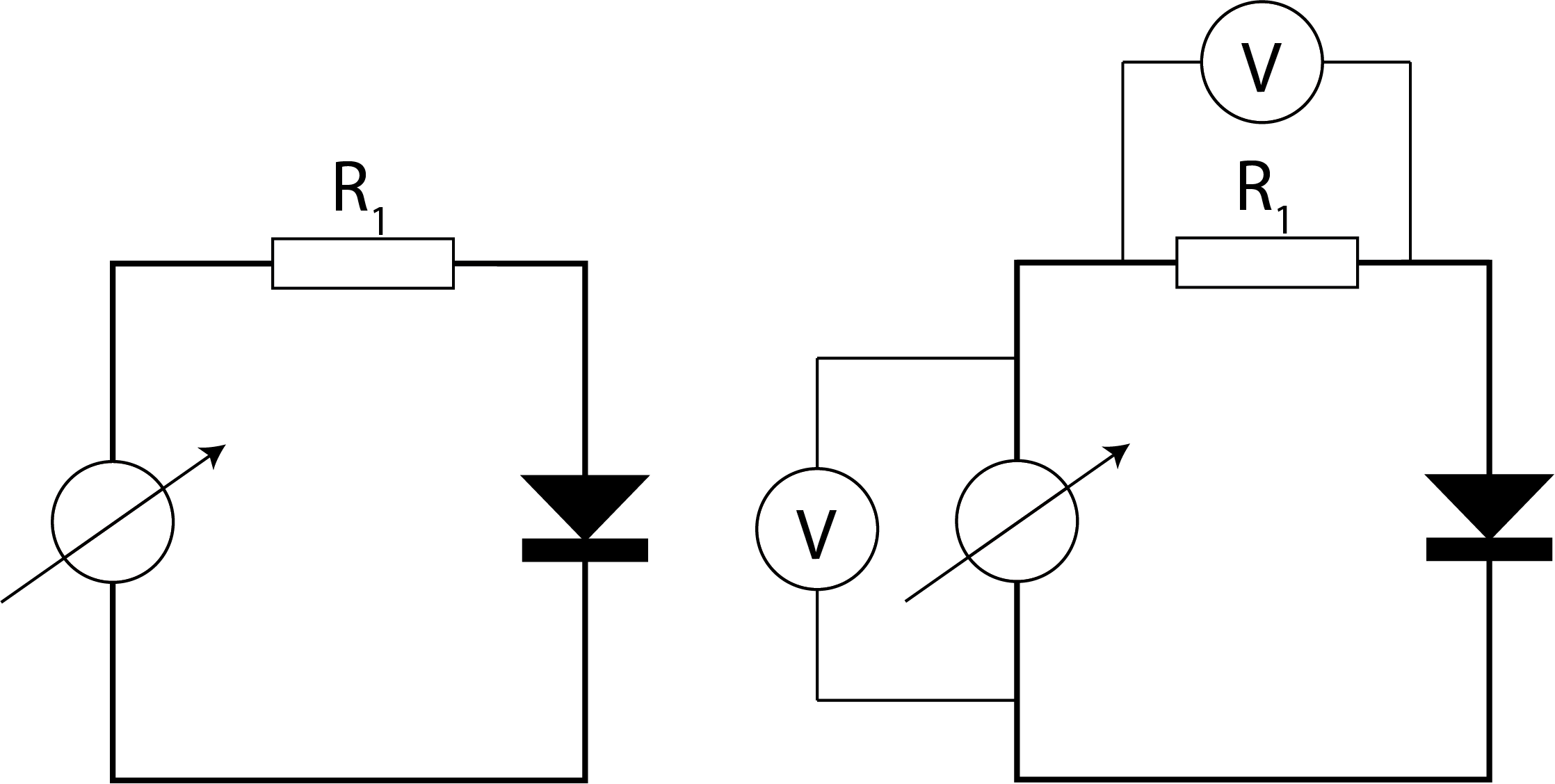
Fig. 4 Measuring voltage already changes the electric ciruit itself.#
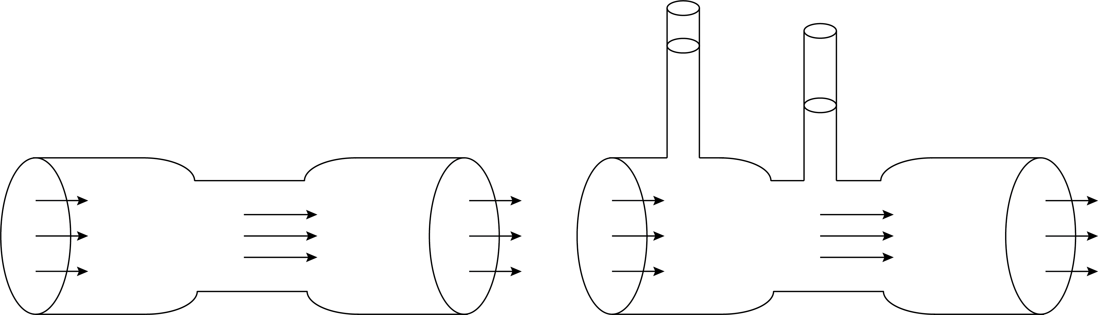
Fig. 5 Placing pressure gauges in a liquid flow affects the original flow.#
Systematic error#
In addition to influencing the measurement of your physical quantity by measuring it, there are other causes that can lead to ‘errors’. We distinguish between systematic errors and random errors. A systematic error will always be the same size, and therefore causes a deviation in your average result. Such an error strongly influences your final result. Fortunately, you can correct for this type of error. Examples of systematic errors are a zero point error and a calibration error, see for example Figure 6.
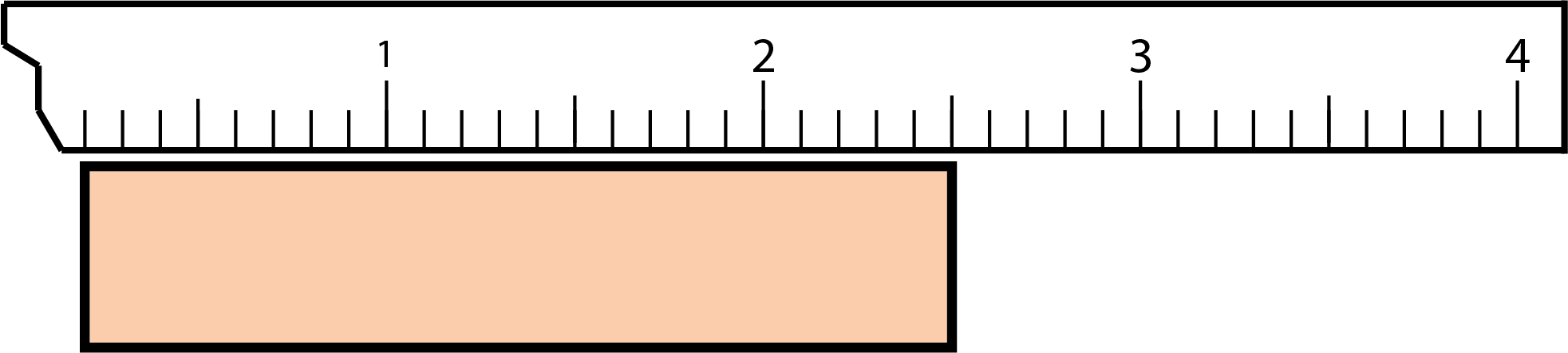
Fig. 6 This creates a systematic error if you are not aware that the ruler does not start at 0.#
To find out whether there is a systematic error in your data, you can check this using Python, for example. This is best explained using an example.
Example: Systematic error
You are conducting research into the influence of distance on force. To do this, you measure the distance, but you are concerned that there may be a systematic error in the distance \(r\) because that distance cannot be measured accurately. If you investigate the expected relationship \(F = \frac{a}{r^4}\), you can try to fit the function \(F = \frac{a}{(r+\Delta r)^4}\). In the ideal situation, without systematic error, \(\Delta r\) is equal to 0. If this formula produces a better fit for \(\Delta r \neq 0\) (Figure 7), then \(\Delta r\) may be your systematic error. Of course, you then need to investigate whether this value is reasonable and can be explained.
In Figure 7, you can see the difference between a fit with and without compensation for systematic error. Although the upper figure appears to be a good fit, you can see that the fit in the lower figure is even better across all measurements. Later, we will look at how we can investigate such errors more systematically.
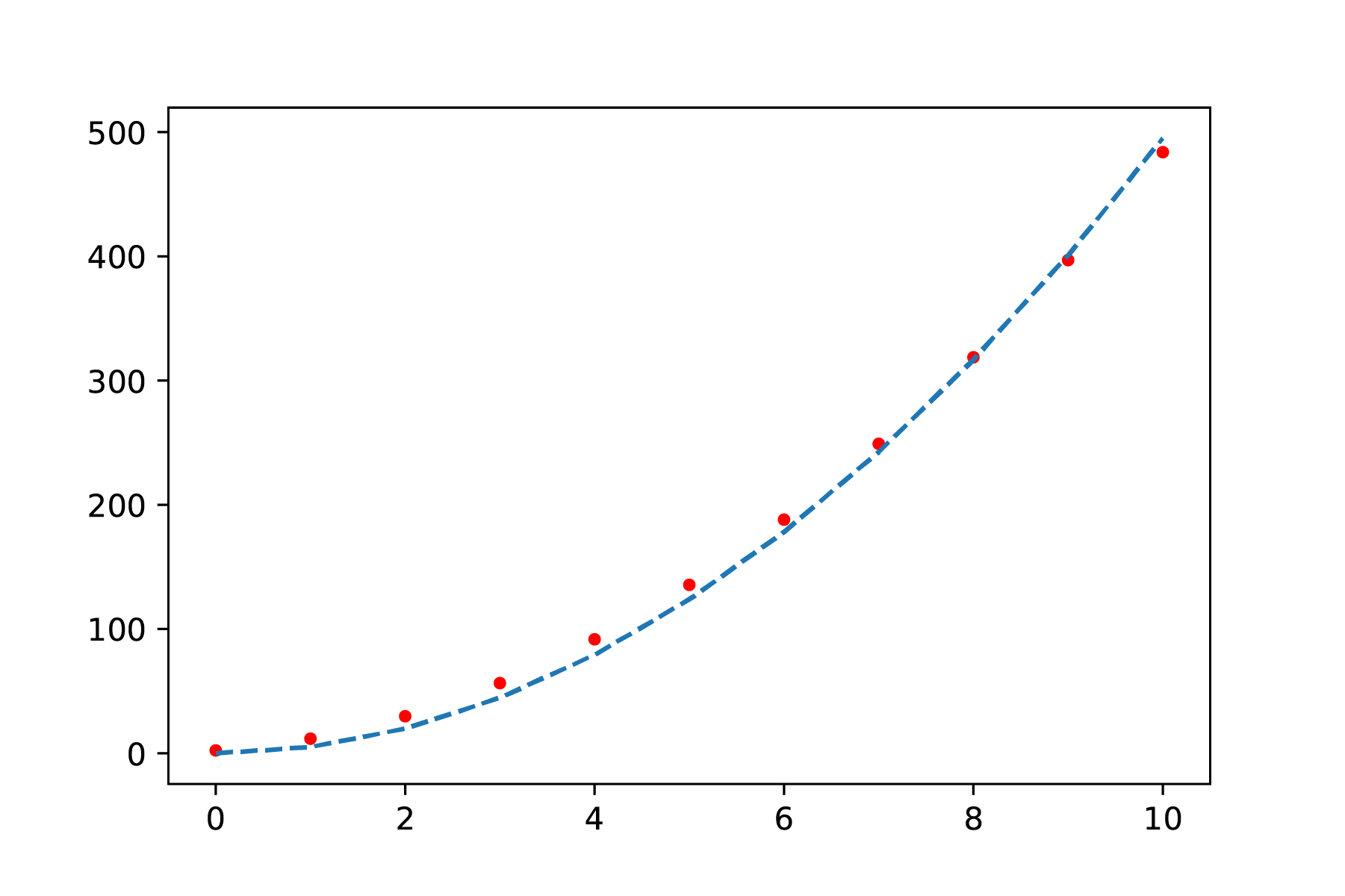
Fig. 7 Least-squares curve fit without correction for the systematic error: \(F = \frac{a}{r^4}\)#
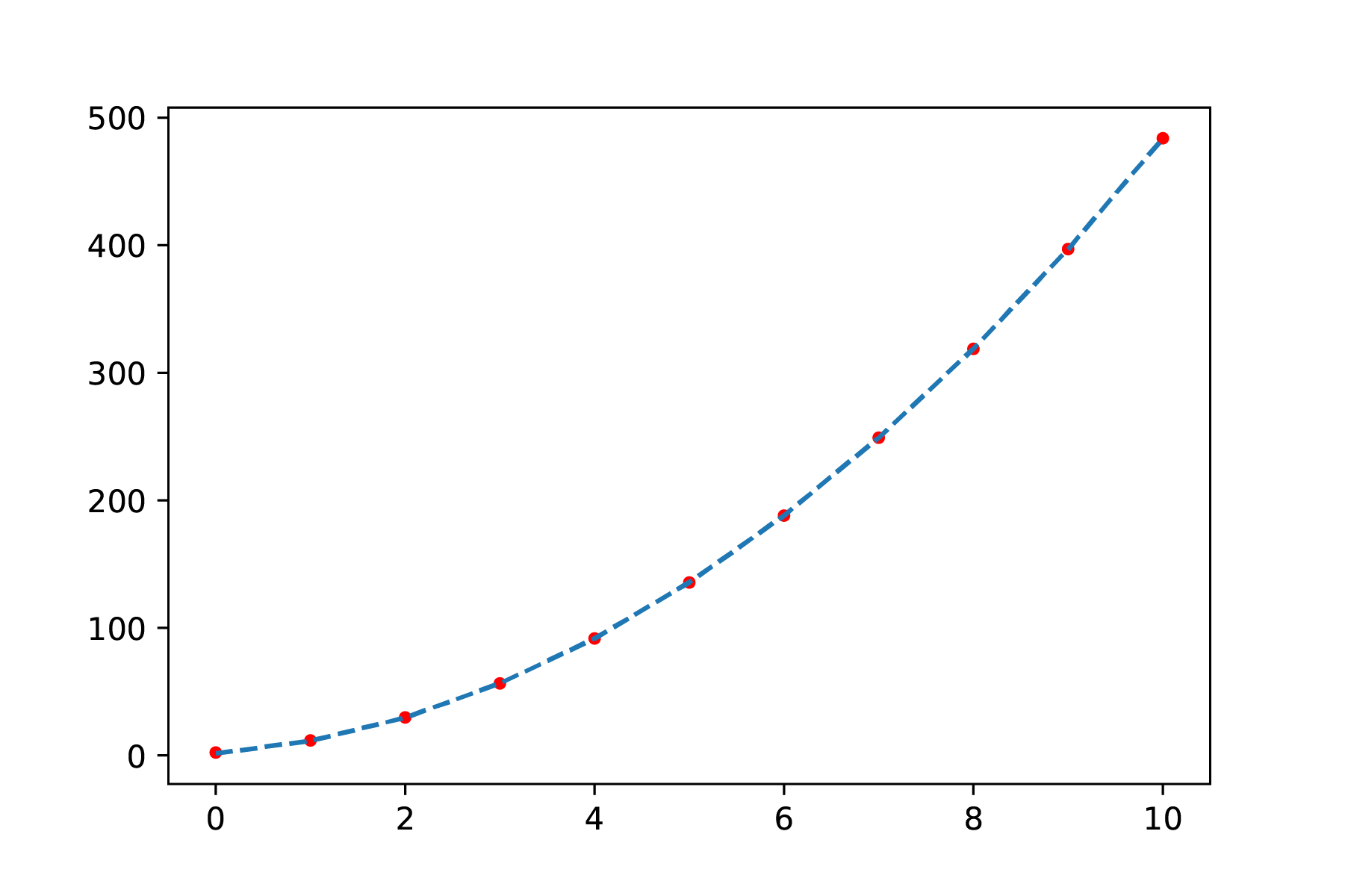
Fig. 8 Least-squares fit with correction for the systematic error: \(F = \frac{a}{(r+\Delta r)^4}\) It is clear that the curve fits with all data.#
Random error#
A random measurement error can arise due to, for example, temperature fluctuations, vibrations, air currents, collisions at the molecular level, etc. This is referred to as a technical random error. These uncertainties cannot always be reduced. Random errors can be both positive and negative, and therefore average out if you take enough measurements. You can work with them and calculate them because they are based on a probability distribution. In the following sections, we assume that you are always dealing with a random error, i.e., an error that is not correlated with other variables and for which the probability of that error occurring is normally (Gaussian) distributed.
In addition to technical random errors, you may encounter fundamental errors due to physical limitations on some measurements, for example due to thermal fluctuations when measuring currents. This is referred to as a fundamental random error. This contribution to the measurement uncertainty cannot be reduced. The contribution to the total uncertainty can be either positive or negative.
Instrumental uncertainties#
Every instrument you use has certain limitations. The uncertainty may be dependent on reading the instrument, but also on the instrument itself, or on the value of the measured quantity. In addition, you must first calibrate (some) instruments before using them. An error in calibration can lead to a systematic error.
When using instruments, the terms precision and accuracy are often used. Precision refers to the small spread in the measurements. Precision is closely related to random errors. Accuracy refers to how close the measurements are to the desired value. Accuracy is closely related to systematic errors. The four variants that you can have are shown in Figure 9.
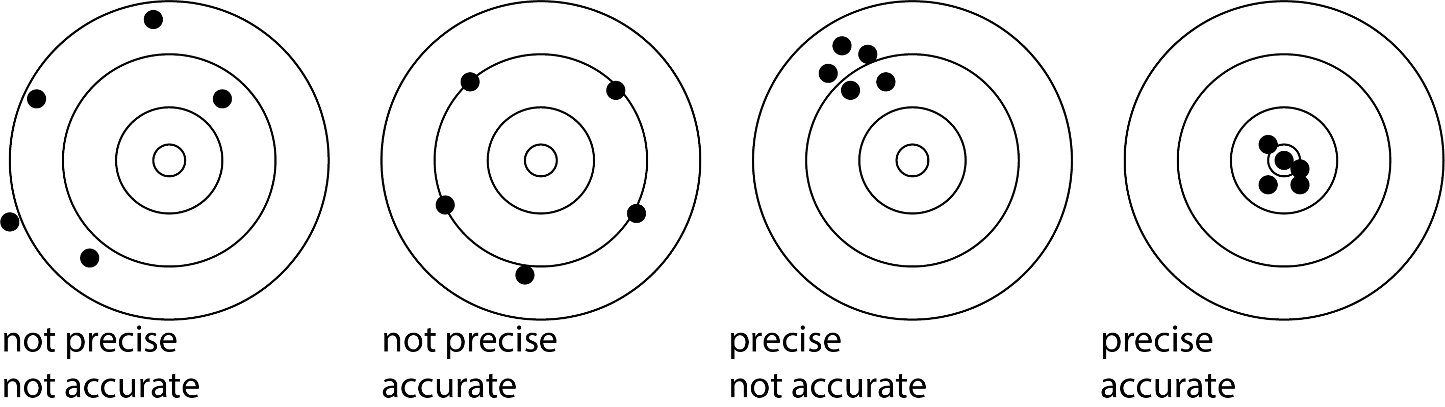
Fig. 9 The four variants concerning accuracy and precision. Accuracy is strongly linked to systematic errors, precision to random errors.#
Measuring scales
Different measuring instruments have different measuring scales. We distinguish between nominal, ordinal, interval, ratio, and cardinal scales.
1. Nominal scale
If we only name the quality of the object, the measuring scale is called nominal. Determining the color of a solution is an example of this.
2. Ordinal scale
If the designation involves a ranking, we refer to an ordinal scale. An example is giving grades for academic performance. Someone with a 10 knows more than someone with a 5, but that person does not know twice as much. Also, the difference in knowledge between a 5 and a 6 is usually incomparable to the difference between a 9 and a 10.
3. Interval scale
A scale on which equal differences mean the same thing but ratios do not, is called an interval scale. On an interval scale, the zero point is arbitrary. The Celsius scale is an example of this. 100 ˚C is not twice as high a temperature as 50 ˚C, but the temperature difference between 50 ˚C and 51 ˚C is the same as between 100 ˚C and 101 ˚C.
4. Ratio scale
If, in addition to differences, we can also use ratios of measurement results in a meaningful way, then the measurement takes place on a ratio scale. Measuring lengths is an example. A table that is 2 m wide is twice as wide as a table that is 1 m wide. We strive to bring measurement to the level of a ratio scale. An example is the transition from the Celsius scale to the absolute temperature scale (the Kelvin scale).
5. Cardinal scale
The fact that we can measure on an interval scale with a fixed zero point or on a ratio scale does not determine the numerical values. Only when we have chosen the unit (for Celsius temperatures the ˚C, for lengths for example the meter) can we assign numerical values. We then speak of a cardinal scale.
Measurement uncertainty in analog instruments
With analog instruments, you have to read the value, see Figure 10. In some cases, there is a mirror behind the pointer so that you don’t make a mistake by reading the pointer at an angle. Furthermore, you cannot read the value with infinite precision. Think of a measuring stick that allows you to measure accurately to the nearest millimeter, but where distances between millimeters cannot be determined accurately, especially when the lines on the ruler are thick. When reading an analog meter, you must estimate the associated uncertainty:
Read the value as accurately as possible.
Determine the values that you can still read accurately.
Then take half of the difference between two values that you can accurately read as a measure of uncertainty.
Example: Interpolating readings
The best reading of the pointer in Figure 10 would be 17.3. The value is clearly between 17 and 17.5, closer to 17.5 than 17. The values 17 and 17.5 would be easy to read. Half of that is 0.25. The uncertainty is then 0.3 (we are not allowed to round down an uncertainty).
As you can see, there are not always fixed rules for determining measurement uncertainty, and sometimes it comes down to common sense and reasoning how you arrive at that value.
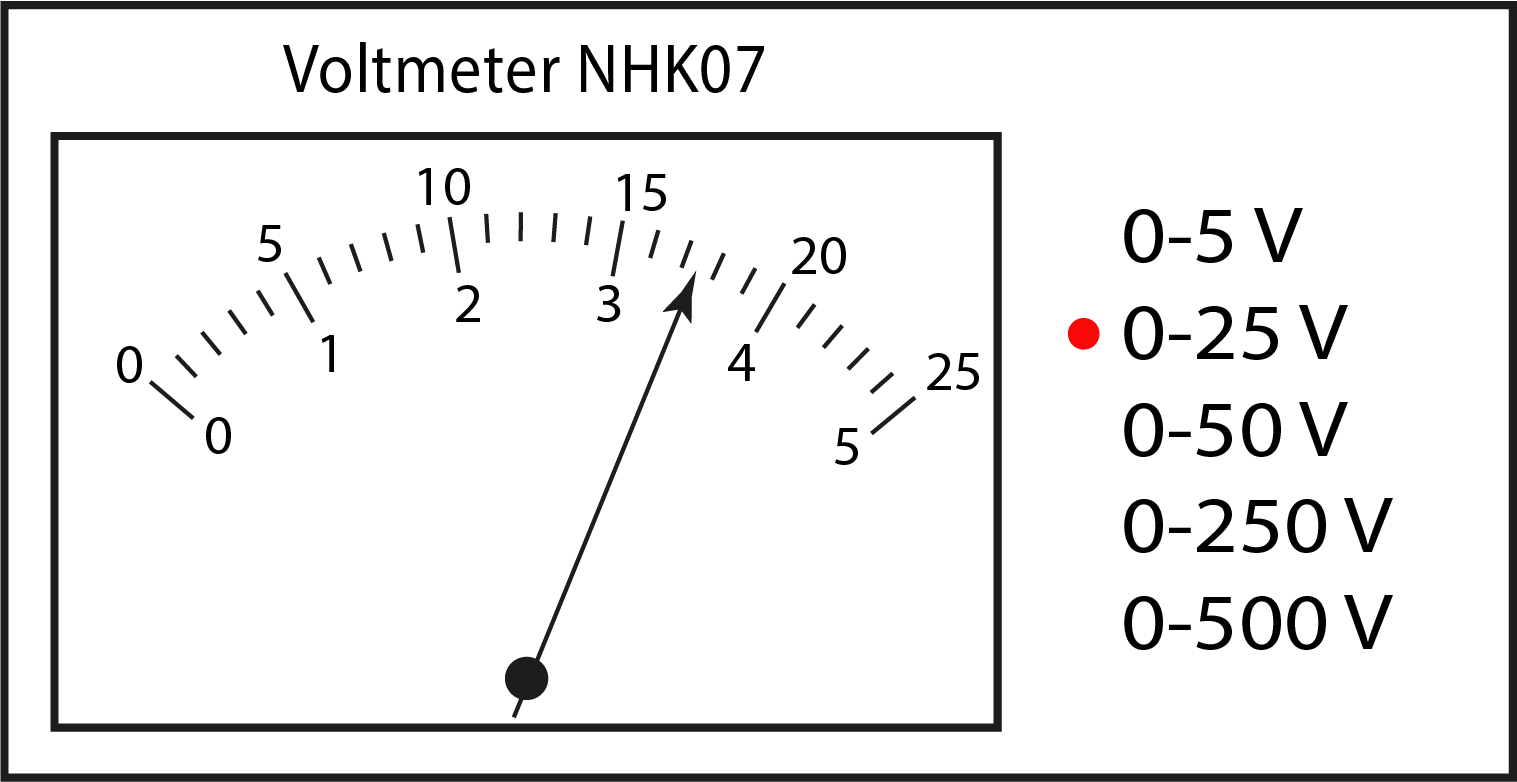
Fig. 10 Reading an analog meter where the first decimal place must be estimated based on interpolation.#
Measurement uncertainty in digital instruments
When reading a digital instrument, see Figure 11, you would say that the uncertainty lies in the last decimal digit shown. However, the uncertainty of digital instruments is much greater than the last decimal digit; just think of the uncertainty when using a stopwatch. For devices used in physics practicals, this uncertainty is sometimes even determined by the age of the device and the time it has been switched on (warming up). For many digital (expensive) devices, the specifications state exactly how the measurement uncertainty should be calculated.
Fig. 11 The digital multimeter determines the “exact” value of a 33 kΩ (5% tolerance) resistor.#
Mean, standard deviation and standard error#
Because measured values can fluctuate, the average of a series of repeated measurements (\(x_i\)) provides the best possible approximation of the actual value. The average value is calculated based on the series of repeated measurements:
Of course, a repeated measurement only makes sense if your instrument is accurate enough to show variations. There is a degree of dispersion in the series of measurements: the measurements differ from each other. The standard deviation is a measure of that dispersion:
Although the mean and standard deviation are better defined with more measurements, the standard deviation does not decrease in value, see Figure 12. The spread itself is therefore not a good measure of the uncertainty in your mean value. The uncertainty in your mean is given by:
An important insight is that the measurement uncertainty decreases with the square root of the number of measurements. To reduce the measurement uncertainty based on multiple measurements by a factor of 10, you need to perform 100 times as many repeated measurements. The optimum number of repeated measurements therefore depends on (1) the accuracy you want to achieve, and (2) the time and money you have available to achieve that accuracy.
Fig. 12 Noise generation shown as points and in a histogram. Bottom left the standard deviation (convergent) and bottom right the measurement uncertainty (decreases with \(\frac{1}{\sqrt{N}}\)).#
The measurement uncertainty is equal to the deviation of the mean of repeated experiments. That is, if the entire experiment is repeated, there will always be a difference in the determined mean. The standard deviation of this mean is equal to \(u(x)\), or, there is a roughly 2/3 chance that when the entire experiment is repeated, the average will lie between \(\overline{x} \pm u(x)\). The code below shows how you could verify this statement.
Tip
To run and modify the code below, press the rocket at the top of the page. After loading the necessary packages, you can get started!
The to be reported value you use is written as:
The uncertainty determines the number of significant digits to be used. You use the same number of decimal digits.
Example: Notation
The average of a repeated measurement is \(4.04 \mathrm{V}\) with an uncertainty of \(0.1 \mathrm{V}\). The uncertainty has 1 significant figure, so you record the measurement as: \((4.0 \pm 0.1) \mathrm{V}\).
Exercise 3
Determine the mean, standard deviation and standard error of the next measurement series:
0.10; 0.15; 0.18; 0.13
25; 26; 30; 27; 19
3.05; 2.75; 3.28; 2.88
Solution to Exercise 3
\(\overline{x}\)=0.14, \(\sigma\) = 0.034, \(u(x)\) = 0.02
\(\overline{x}\)=25.4, \(\sigma\) = 4.0, \(u(x)\) = 2
\(\overline{x}\)=2.99, \(\sigma\) = .23, \(u(x)\) = 0.1
Weighted average#
It may happen that not all repeated measurements are equally reliable. If measurement 1 has half the uncertainty of measurement 2, then it seems logical that the average is calculated by \(\frac{2 \cdot x_1 + 1 \cdot x_2}{3}\). We then refer to this as a weighted average. The question is, of course, how to determine the reliability and how to arrive at our weighting factor. Fortunately, we have just found a measure for this, namely the measurement uncertainty. The weighting factor is defined by:
The weighted average becomes:
with an associated uncertainty of:
Note that the above formula reduces to the normal mean if all weighting factors \(w_i\) are equal to 1.
Exercise 4
In an experiment during physics lab, the acceleration due to gravity is determined. This yields the following values for different groups: 9.814 ± 0.007, 9.807 ± 0.003, 9.813 ± 0.004.
Calculate the weighted average and the corresponding uncertainty.
Solution to Exercise 4
9.809 ± 0.002 m/s²
Note that the uncertainty in the final answer has decreased!
Probability distributions#
As indicated, there is variation in repeated measurements. We can view the physical measurement \(M\) as the sum of the physical value \(G\) and noise \(s\):
Noise is broadly defined here; we understand it to mean all possible errors. We are particularly interested in random errors. These are normally distributed.
Gaussian distribution#
When dealing with random noise, the probability of a value occurring can be described using a normal (Gaussian) distribution:
Here, \(P(x)\) is the probability density function, with \(\mu\) being the mean value of the noise and \(\sigma\) being the standard deviation.
An example of a noise signal is shown in Figure 13 (the corresponding code is shown in a cell below). The mean of these values is 0. Repeating measurements therefore limits the influence of the noise because the mean contribution is 0:
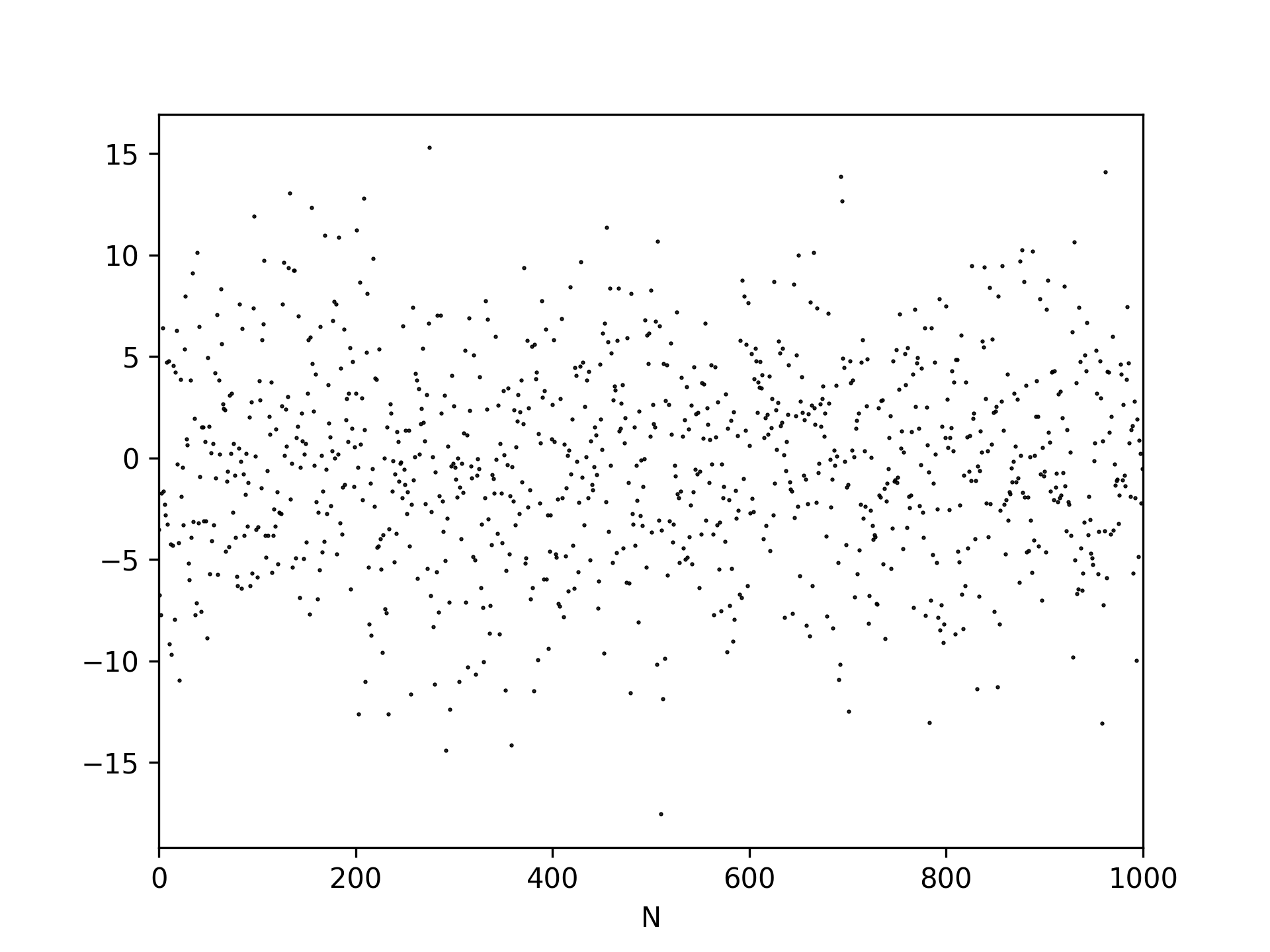
Fig. 13 Random noise, observe that outliers exist but are not frequent.#
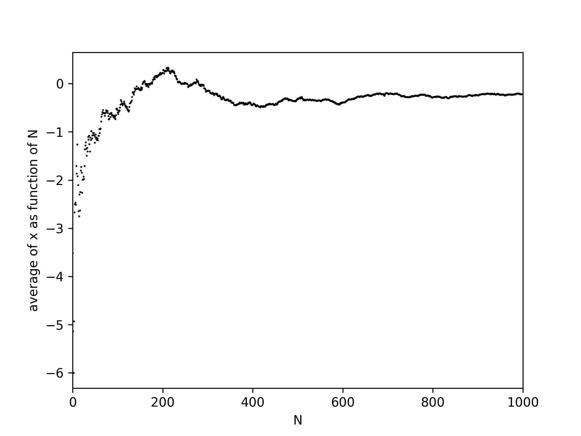
Fig. 14 The average value of noise is increasingly well defined with repeated measurements.#
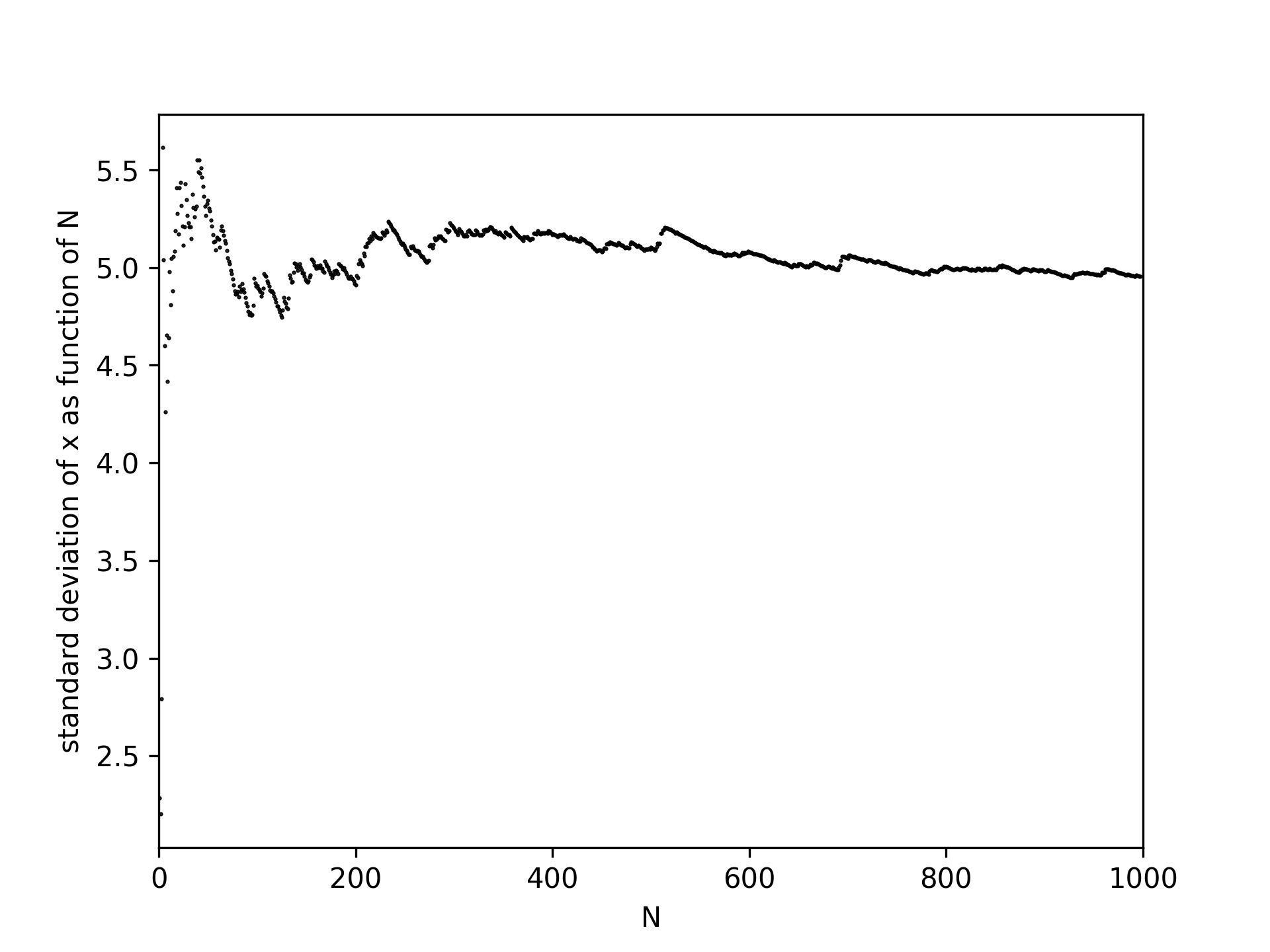
Fig. 15 The standard deviation becomes increasingly well defined with repeated measurements.#
We must be careful here, as Figure 16 shows that a histogram of four repeated measurements of noise always gives a slightly different picture. Each histogram consists of 1000 repeated measurements. So there is even an uncertainty in the uncertainty \(\left( \frac{1}{\sqrt{2N-2}}\right )\). The exact way in which we report our values is elaborated in Measurement uncertainty and significant figures.
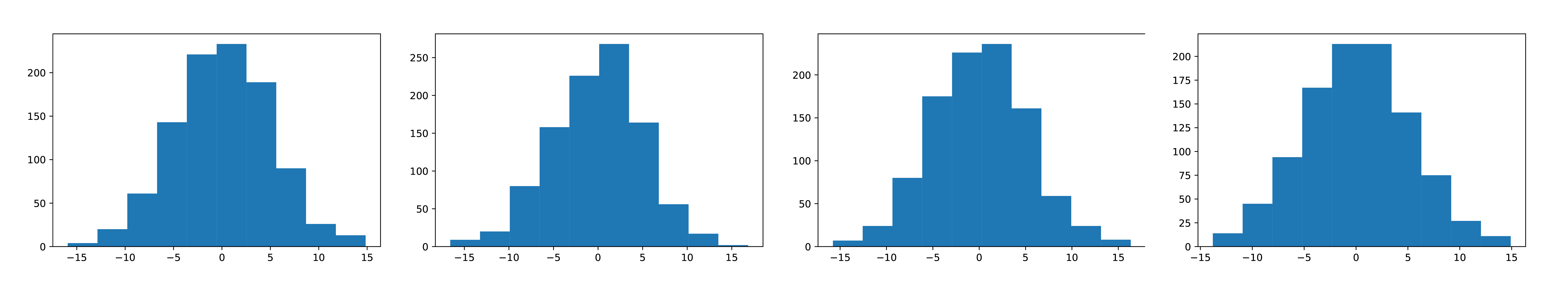
Fig. 16 Even 1,000 repeated measurements (of noise) show differences.#
Below you can ‘play’ with the mean value and the standard deviation to see how these influence the measurements.
<function __main__.update(average_value, std_value)>
# we voeren hier een experiment met 1000 samples 100x uit. Als bovenstaande klopt, dan is de standaard deviatie in het gemiddelde van de verschillende experimenten gelijk aan de onzekerheid in een enkele dataset.


mean_values = np.array([])
N = 100
samples = 1000

for i in range(N):
    dataset = np.random.normal(1.00,0.5,samples)
    mean_values = np.append(mean_values,np.mean(dataset))

print('The standard deviation in the mean of repeated experiments is: ', np.std(mean_values,ddof=1))
print('The uncertainty in a single dataset is: ', np.std(dataset,ddof=1)/np.sqrt(samples))
The standard deviation in the mean of repeated experiments is:  0.015551291350132876
The uncertainty in a single dataset is:  0.01610524973279738
Poisson distribution#
A second probability distribution we introduce here is the Poisson distribution. Unlike the normal distribution, the Poisson distribution is discrete. It is used to count independent events within a certain time interval, where the events themselves occur randomly. Examples of this are radioactive decay, the number of photons that fall on a detector, etc.
The probability of \(k\) events within a certain time with an average of \(\lambda\) is given by:
The standard deviation in a Poisson distribution is equal to the square root of the mean (\(\sigma = \sqrt{\lambda}\)).
Example: Poisson
An average of 20 people eat at a restaurant every day. What does the probability distribution of the number of people who come to eat look like?
The probability distribution of the number of visitors is shown in Figure 17. The probability is described by: \(P(X = k) = \frac{20^k e^{-20}}{k!}\).
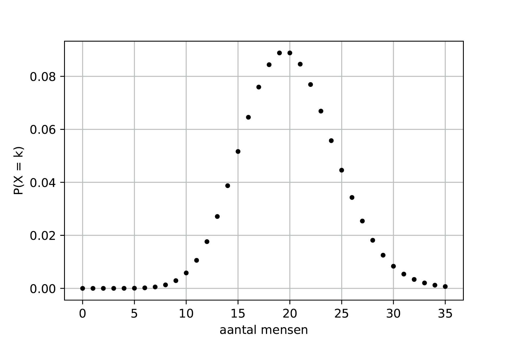
Fig. 17 The probability distribution of the number of visitors to the restaurant.#
Both the shape and the function are somewhat similar to those of the Gaussian distribution. However, there are clear differences, particularly for small values of \(\lambda\). Furthermore, the number of events is always at least 0, whereas in a Gaussian distribution, the expected value can also be less than 0.
Uniform distribution#
When you roll a die, the probability of rolling a 1 is the same as rolling a 6. In other words, the probability for any random number is uniformly (discreetly) distributed. Now suppose we are dealing with a continuous, uniform probability distribution, then the probability density function applies:
The probability that a point lies between the values \(X\) and \(X+dX\) (if \(X\) lies between \(a\) and \(b\)!) is then given by:
The expected value is simply being calculated by:
and its standard deviation by:
Monte Carlo simulation#
Such a uniform distribution is useful in Monte Carlo simulations, for example. In such a simulation, a large number of random points are generated and then examined to see where they end up. For an integral that cannot be solved analytically, you can still calculate the surface area:
Here, \(y_{min}\) and \(y_{max}\) are the vertical limits you choose for creating your random points. Of course, these must cover the entire graph!
An example of a Monte Carlo simulation is given in Figure 18, in which a simple integral is calculated by determining whether \(y<x^2\) applies for 10,000 points. The integral on the domain [0,5] is then equal to the number of points that satisfy this condition divided by the total number of points created times 5 times 25. In such a Monte Carlo simulation (which is a counting problem), the uncertainty scales with \(\frac{1}{\sqrt{N}}\), where \(N\) is the number of points that satisfy the condition (so choose the vertical boundaries optimally!).
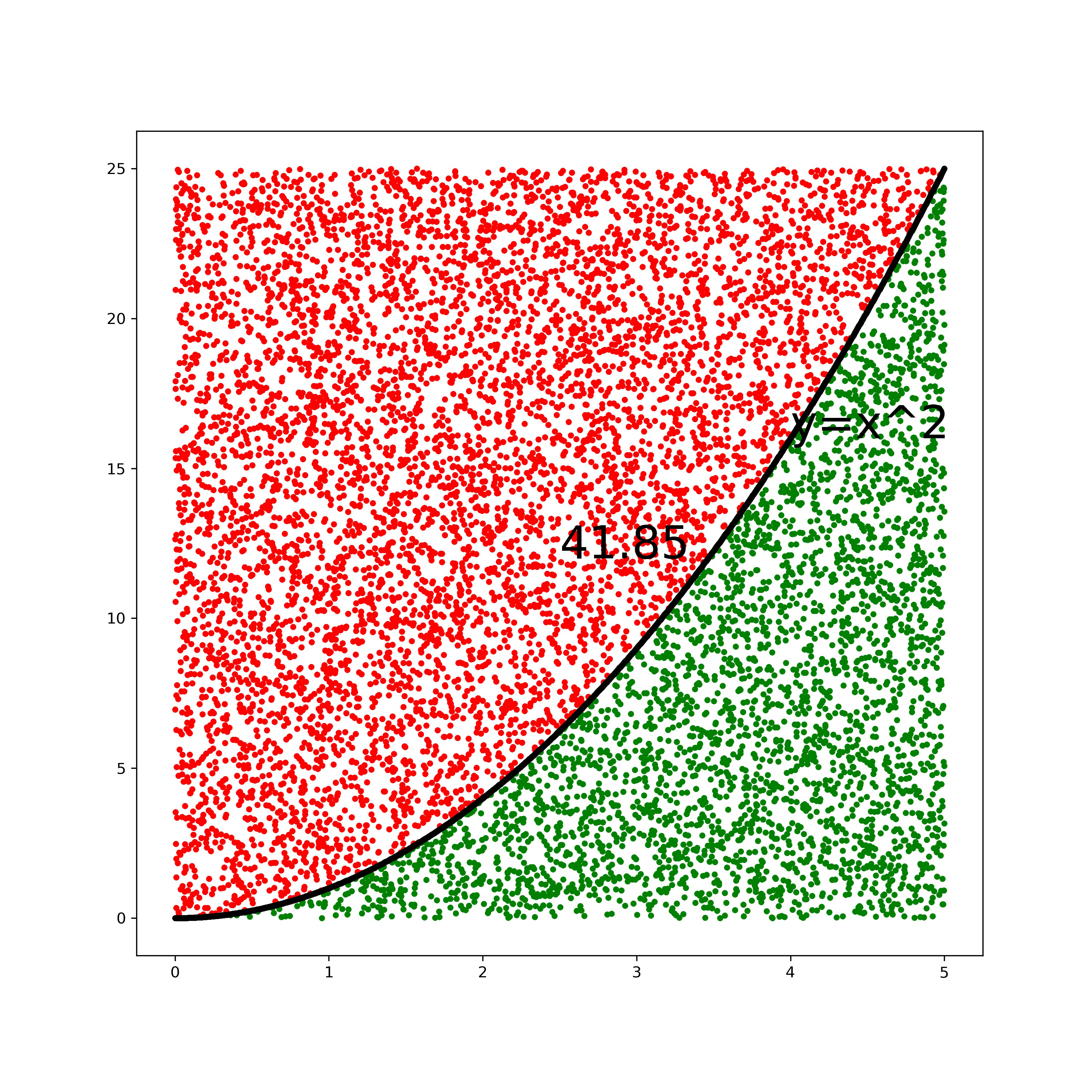
Fig. 18 An example of a Monte Carlo simulation for calculating an integral using a uniform distribution of random points.#
Chauvenet’s criterium#
Repeated measurements lead to a better average. However, in repeated measurements, certain values can deviate significantly from the average. It can be tempting to simply write off a measurement point that deviates significantly from the rest as a measurement error. However, this quickly becomes data manipulation, which is not the intention. You can apply Chauvenet’s criterion to see if the measurement point can be removed. Chauvenet’s criterion is a rule of thumb (there are other, more complicated methods for determining whether you can remove data points, but we will not discuss them here). Chauvenet’s criterion states that a measurement may be removed from the dataset if the probability of this is less than \(\frac{1}{2N}\) or \(P(X)<\frac{1}{2N}\).
In more detail, this means that you first calculate the mean and standard deviation of your data, including the suspicious point. You can then omit a point if it satisfies the following inequality:
where
Here, erf is the error function, the integral of the normal distribution. The result of this integral cannot be calculated algebraically. You can calculate the value for the error function at https://www.danielsoper.com/statcalc/calculator.aspx?id=53. Below, we explain how to do this in Python.
If you use Chauvenet’s criterion to exclude an outlier, you must always mention this in your report! In addition, you must recalculate the mean and standard deviation after removing the suspect point. After all, this point has a significant effect on your dataset.
Exercise 5 (Outlier)
Which measurement from exercise 3 series 2 is suspicious? Use Chauvenet’s criterion to see if you can exclude this measurement.
Solution to Exercise 5 (Outlier)
\(P_{out} = 2\cdot \text{Erf}(x = 19,\overline{x} = 25.4,\sigma = 4.0) = 2 \cdot 0.05479929\)
\(N\cdot P_{out} = 0.5479929 > 0.5\). We can not discard the measurement.
Error function(s)#
There are two kinds of error functions, the \(\text{erf}(x)\) and the \(\text{Erf} \space (x_{out},\overline{x},\sigma)\) (also called the cdf function). These are defined as:
A plot of both functions is given in Figuur 19
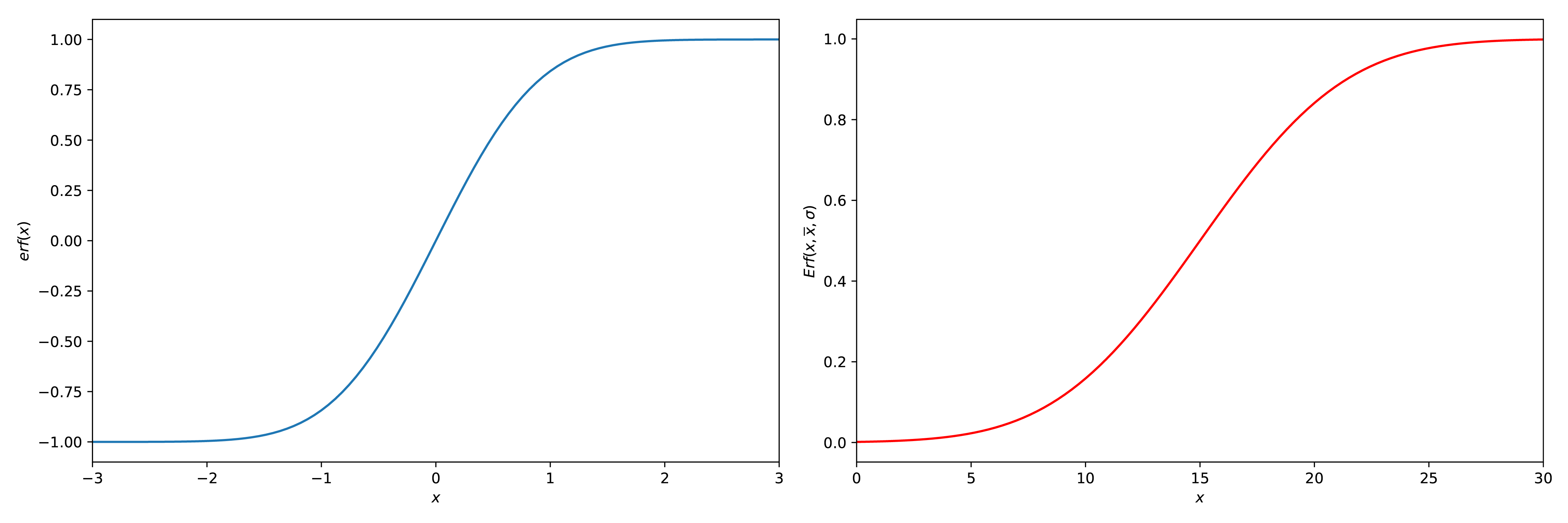
Fig. 19 2 plots, one with \(\text{erf}(x)\) (left) and one with \(\text{Erf}(x_{out},\overline{x},\sigma)\) (right), \(\overline{x} = 10\) and \(\sigma = 5\).#
Both functions can be found in the scipy.special.erf and scipy.stats.norm.cdf functions. When using the Erf or scipy.stats.norm.cdf function (or the site), keep in mind that when investigating an upward outlier, the functions will all return a value above 0.5. This means that you must do \(P_{out\_new} = 1 - P_{out}\). The final code should therefore be something like this:
from scipy.stats import norm

#P is the dataset (a numpy array)
x_out = np.max(P) #In this case, could also have been other outliers
x_mean = np.mean(P)
x_std = np.std(P,ddof=1)

#Use the Erf function
Q = norm.cdf(x_out,x_mean,x_std)
---------------------------------------------------------------------------
NameError                                 Traceback (most recent call last)
Cell In[6], line 4
      1 from scipy.stats import norm
      3 #P is the dataset (a numpy array)
----> 4 x_out = np.max(P) #In this case, could also have been other outliers
      5 x_mean = np.mean(P)
      6 x_std = np.std(P,ddof=1)

NameError: name 'P' is not defined
#You could have also defined the Erf on your own

#Check if it is a high 'outlier'
if Q > 0.5:
    Q = (1-Q)

#Use Chauvenets criterion
C =  2 * len(P) * Q

if C < 0.5:
    print('The value can be discarded.')
else:
    print('The value cannot be discarded.')
Measurement uncertainty and significant figures#
An important rule regarding significant figures is that you must first determine the number of decimal places in your uncertainty. If you have fewer than \(10^4\) measurement points, the uncertainty should be expressed with one significant digit. The significance of your result is then adjusted so that its last digit corresponds to the digit of the uncertainty. You can use powers of 10 or prefixes to clearly represent the number, see table below.
Example:
Question:
Determine the mean value (including its uncertainty) of the measurement series.
Measurement |
\(U\) (V) |
1 |
5.050 |
2 |
4.980 |
3 |
5.000 |
4 |
4.950 |
5 |
5.020 |
Answer:
First, we determine the mean value \(\mu_U=\overline{U}=\frac{1}{N}\sum_{i=1}^{N} U_i = 5.000 \mathrm{V}\).
Then we determine the standard deviation \(\sigma(U) = \sqrt{\frac{1}{N-1}\sum_{i=1}^N (U_i-\overline{U})^2} = 0.038078866 \mathrm{V}\).
Finally, we determine the uncertainty in the average value \(u(U) = \frac{\sigma(U)} {\sqrt{N}} = 0.017029386 \mathrm{V}\).
We have fewer than \(10^4\) measurement points, so we round the uncertainty to 1 significant figure: \(u(U) = 0.02 \mathrm{V}\).
The uncertainty has two decimal places, so we adjust our mean accordingly: \(\overline{U} = 5.00 \pm 0.02 \mathrm{V}\).
There is another important point regarding rounding. If you were to round all fives up, you would introduce a systematic error; you always round up. The agreement is that if the number before the \(5\) is even, you round down (\(33.45 \rightarrow 33.4\)), and if the number before the \(5\) is odd, you round up (\(33.55 \rightarrow 33.6\)). In addition, in some fields it is good practice not to round down the uncertainty, as this prevents underestimating the uncertainty. However, we do not take this into account in physics practicals.
Table: Powers of 10, including their symbols.
power of 10 |
\(10^{-12}\) |
\(10^{-9}\) |
\(10^{-6}\) |
\(10^{-3}\) |
\(10^{-2}\) |
\(10^{-1}\) |
\(10^1\) |
\(10^2\) |
\(10^3\) |
\(10^6\) |
\(10^9\) |
\(10^{12}\) |
|---|---|---|---|---|---|---|---|---|---|---|---|---|
prefox |
pico |
nano |
micro |
milli |
centi |
deci |
deca |
hecto |
kilo |
mega |
giga |
tera |
symbol |
p |
n |
\(\mu\) |
m |
c |
d |
da |
h |
k |
M |
G |
T |
For additional information about significant figures, you can watch this video.
Errorpropagation#
You often apply a calculation to your raw data to arrive at an answer to your research question. A small deviation in your measurement can have major consequences for your final answer. That is why it is important to take the impact of uncertainties into account. There are two methods for calculating errors: the functional approach and the calculus approach. The former is more intuitive, but the latter is slightly easier to calculate.
In the theory below, we assume that we apply a function \(Z\) to our empirically determined value \(x\), whose mean is \(\overline{x}\) with an uncertainty \(u(x)\).
Functional approach#
With the functional approach, you look at the difference when you evaluate the function at the point that is one uncertainty away from your measuring point. In formula form, this becomes:
In many cases, symmetry applies, which means that the above equation can also be interpreted as:
Example:
Question:
Calculate the circumference of a circle with a radius of \(r = 2 \pm 0.1 \) cm
Answer:
\(O = 2\pi r = 4.0\pi \approx 12.5664 \) cm
\(u(O) = \frac{O(2+0.1) - O(2-0.1)}{2} = 2\pi\frac{2.1-1.9}{2} \approx 0.628...\)cm
\(O = 12.6 \pm 0.6\)cm
The functional approach is very useful for calculations that you need to repeat. In Python, you first define the function and then calculate the outcome for the variables + uncertainty. See the code below for the example given. This saves you a lot of time and calculations. However, when setting up a new method, the calculus approach gives a better picture of the magnitude of the uncertainties. You can use the calculus approach to dimension your experiment.
# Functional approach in calculation uncertainty of circumference of a circle
import numpy as np
def omtrek(x,a):
    return 2*np.pi*(x+a)

r = 2.0
ur = 0.1

u_omtrek = (omtrek(r,ur)-omtrek(r,-ur))/2
print(u_omtrek)
Calculus approach#
In the calculus method, you use partial derivatives to linearize the effect of an error:
A consequence of the linear approach to the error is that this method becomes less accurate as the error increases or the function exhibits strongly non-linear behavior.
Example:
Question:
Determine the equation of the uncertainty in \(f(x) = 2x\cos{x}\)?
Answer:
We make use of the calculus approach. To do this, we determine the derivative of \(f(x)\) to \(x\).
Next, we apply the calculus approach:
Multiple variables#
If your result is a function of multiple independent variables, you add the errors quadratically:
Using the calculus method, it can be deduced that the uncertainty \(u(f)\) applies to a function \(f(y,x)=cy^nx^m\):
Exercise 6
Eric is weighing a box. The mass is (56 \(\pm\) 2) g. The box’s sides are (3.0 \(\pm\) 0.1) cm.
Calculate the gravity working on the box.
Calculate the volume of the box.
Calculate the density of the box.
Solution to Exercise 6
\((0.55 \pm 0.02) \) N
\((27 \pm 3)\) cm\(^3\)
\((2.1 \pm 0.2) \) g/cm\(^3\)
Example:
Question:
Calculate the uncertainty in \(g(x,y) = \ln(x)e^{2y}\)
Answer:
We use the calculus approach. To do this, we determine the partial derivatives of \(g(x)\) to \(x\) and \(y\).
Next, we add those uncertainties quadratically:
Tip: Standard functions
Tabel: Overview of widely used functions and the corresponding uncertainties.
Function \(Z(x,y)\)
\(\frac{dZ}{dx}\)
Uncertainty \(u(Z)\)
\(x + y\)
1
\(\sqrt{u(x)^2+u(y)^2}\)
\(x \cdot y\)
y
\(\sqrt{(y\cdot u(x))^2+(x\cdot u(y))^2}\)
\(x^n\)
\(n\cdot x^{n-1}\)
\(\vert n\cdot x^{n-1}\cdot u(x)\vert\) and \(\vert\frac{u(Z)}{Z}\vert = \vert n\frac{u(x)}{x}\vert\)
\(e^{cx}\)
\(ce^{cx}\)
\(\vertce^x \cdot(cx)\vert \cdot u(x)\) or \(\vert c\cdot Z \vert\cdot u(x)\)
\(n^x\)
\(n^x \ln{n}\)
\(\vertn^x \ln{n} \vert\cdot u(x)\)
\(\ln{x}\)
\(\frac{1}{x}\)
\(\frac{u(x)}{\vert x\vert}\)
\(\sin{x}\)
\(\cos{x}\)
\(\vert\cos{x}\vert\cdot u(x)\)
\(\cos{x}\)
\(-\sin{x}\)
\(\vert\sin{x}\vert\cdot u(x)\)
\(\tan{x}\)
\(1+\tan^2{x}\)
\((1+\tan^2{x})\cdot u(x)\) or \((1+Z^2) \cdot u(x)\)
Tip: Calculation rules
Reminder:
Function
Derivative
\(f(x)\cdot g(x)\)
\(f'(x)g(x) + f(x)g'(x)\)
\(\frac{f(x)}{g(x)}\)
\(\frac{g(x)f'(x)-f(x)g'(x)}{g'(x)^2}\)
\(f(g(x))\)
\(f'(g(x))g'(x)\)
Please note that if you have two values A and B that are close to each other and you subtract them from each other (A-B), your error may well be much greater than the difference between those two values. In such cases, you will need to look for alternative measurement methods that yield a smaller relative uncertainty. See below for an example for inspiration.
Example: reducing measurement uncertainty
For an experiment, we want to determine the frequency difference \(\Delta f\) between two tones \(f_0\) and \(f_1\). After a measurement, it turns out that \(f_0 = (1250 \pm 3)\) Hz and \(f_1 = (1248 \pm 4)\) Hz. The difference (including uncertainty) is therefore \(\Delta f = (2 \pm 5)\) Hz (check).
When subtracting values that are close together, there is a chance that the uncertainty is greater than the determined value itself. We can therefore hardly draw any valid conclusions. In such situations, it is necessary to consider alternative ways of measuring the same thing. In this case, this can be done, for example, by using the physical phenomenon of beat. By determining the oscillation period, you can easily determine the frequency difference.
Fig. 20 Time dependent measurement of separate signals.#
Fig. 21 An alternative method to determine the frequency difference of two signals. Sum of both signals. The frequency difference is twice the frequency of the cover of the sum.
Exercise 7
The table below gives measurements of the voltage of and current through a lamp.
Tabel: Measurements of a lamp.
\(U\)(V) |
\(u(U)\)(V) |
\(I\)(mA) |
\(u(I)\)(mA) |
|---|---|---|---|
6.0 |
0.2 |
0.25 |
0.1 |
1.  Determine the power that the lamp absorps.

2.  Determine the resistance of the lamp.

3.  If you could measure either the voltage or the current more accurately, which would you choose and why?
Solution to Exercise 7
\(P = (1.5 \pm 0.6\cdot 10^{-3})\) W
\(R = (2.4 \pm 1\cdot 10^4) \Omega\)
The current, because it has the biggest relative uncertainty.
Exercise 8
The table below gives values and uncertainties for variables \(A\), \(B\), and \(C\). Calculate the value and uncertainties of \(Z\) for the cases given below.
Tabel: Three variables and their uncertainties.
\(A\) |
\(u(A)\) |
\(B\) |
\(u(B)\) |
\(C\) |
\(u(C)\) |
|---|---|---|---|---|---|
5.0 |
0.1 |
500 |
2 |
1 |
0.1 |
\(Z = \frac{A}{BC^2}\)
\(Z = \frac{A}{BC^4}\)
\(Z = C\sqrt{AB}\)
Solution to Exercise 8
\(Z = 0.010 \pm 0.002\)
\(Z = 0.010 \pm 0.004\)
\(Z = 50 \pm 5\)
Dimensioning#
One advantage of the Calculus method over the Functional Approach is that it allows you to dimension your experiment: based on predefined criteria, you can determine how large the experiment should be, what characteristics it should have, and where most of the time and attention should be focused to ensure the experiment meets the set criteria. The easiest way to illustrate this is with an example.
Example:
You want to use a mass-spring system to accurately determine the mass of 10 different loads. The manufacturer states that these loads have a mass of (50 ± 3) g. However, you want to know the exact mass of each load, accurate to the nearest gram. The maximum relative uncertainty is therefore 2%. What does the experiment look like?
The mass of the mass-spring system is calculated as follows:
The uncertainty in the mass is then given by:
The mass is here the mass of the weight on the spring \(m_w\) and an unknown part of the mass of the spring \(m_C\) itself:
The uncertainty in the mass of the weight is then given by:
Based on this comparison and the requirement that \(u(M_w)^2 < 1\)g and the knowledge that \(m\approx50\)g, the experiment can be further dimensioned. Since the spring constant \(C\) and the contribution of the mass of the spring \(m_C\) can be determined in advance, the number of periods to be determined follows from this equation. This knowledge is applied in particular in the open research at the end of this course and in the course Design Engineering for Physicists (DEF) in the following semester. Whereas in the practical course you work towards carrying out the experiment, in DEF you would set requirements for the spring: how accurately must the spring be made (i.e., what is the tolerance you require from the spring manufacturer).
Fitting#
We often measure a quantity as a function of another quantity—for example, the extension of a spring as a function of the applied load, or the period of a pendulum as a function of its length. The purpose of such measurements can vary. For example, we may ask ourselves: How (according to which functional relationship) does the elongation depend on the load? Or: What is the spring constant of the spring? We then assume a certain relationship and use that relationship to determine the values of parameters. In the first case, we refer to this as modeling, and in the second case, as adjusting or “fitting.” In statistics, the second case is known as a regression problem. We will discuss this in more detail below.
Fitting is a procedure that attempts to find a mathematical relationship in a number of (measurement) points. We are then looking for a relationship \(F(x)\) that describes the measurement points \(M(x)\) in such a way that:
First, you need to choose a type of relationship. Examples include a linear fit, a polynomial, sine, etc. In the fitting procedure itself, the parameters of this relationship are chosen so that they best match the data. For example, if a second-order polynomial is being fitted, you look for the combination of \(a\), \(b\), and \(c\) that ensures that the curve \(a + bx + cx^2\) fits your measurement points as closely as possible.
A commonly used method for determining the goodness of a fit is the least-squares method. In this method, the sum of the squared distances from the measurement points to the fit is minimized. To do this, we first define the distance between the measurement point and the fit:
This distance is also referred to as the residue, which we will discuss in more detail later. The total sum of the absolute distances must be as small as possible:
Fig. 22 The idea of a least-square method is that the area is minimized.#
You can see when \(\chi^2\) is as small as possible by playing with the sliders below.
In the above case, we assume that the value of the independent variable has been determined with sufficient accuracy and precision. There are other techniques that take into account the deviation in the dependent variable. We can also look again at the influence of measurement uncertainty in determining the best fit.
Weighted fit#
Just as a weighted average takes into account the uncertainty in the measurement, you can use a weighted fit for a function fit. This allows you to take into account the uncertainty in the dependent variable (there is also a technique that takes into account the uncertainty in both the independent and dependent variables, but we will not discuss that here).
For a weighted fit, the smallest value for \(\chi^2\) is considered, taking the uncertainty into account:
Other fit types#
In a least-squares fit, we attempt to minimize the squared residuals. This method works particularly well when the uncertainty is primarily in the dependent variable. In such cases, we can control the independent variable or reduce its uncertainty enough that it becomes negligible compared to the uncertainty in the dependent variable.
However, the least-squares method is not the only fitting approach. There is also, for example, the ‘orthogonal distance regression’ method, also called smallest distance method. This method is visualized in Figure 23. We will not provide the further mathematical elaboration here, but how the method can be implemented can be found in source.
Fig. 23 Another fitting method is ODR, which minimizes the distance to the fitting line.#
Residual analysis#
In one of the previous sections, we discussed that a physical measurement (\(M(x)\)) can be described as the sum of the physical value (\(G(x)\)) + noise (\(s\)). A function fit (\(F(x)\)) is performed based on the measurements. To check that we have a good fit, we need to look at the noise. We would get this if we subtract the fit function from the measurement:
The initial analysis is performed by plotting the noise \(s\) as a function of the independent variable \(x\). If there is a pattern in this, for example a rising line, a sinusoidal signal, or all noise points above 0, see Figure 24, then there is a good chance that a better function \(F(x)\) can be found that describes the physical value \(G(x)\).
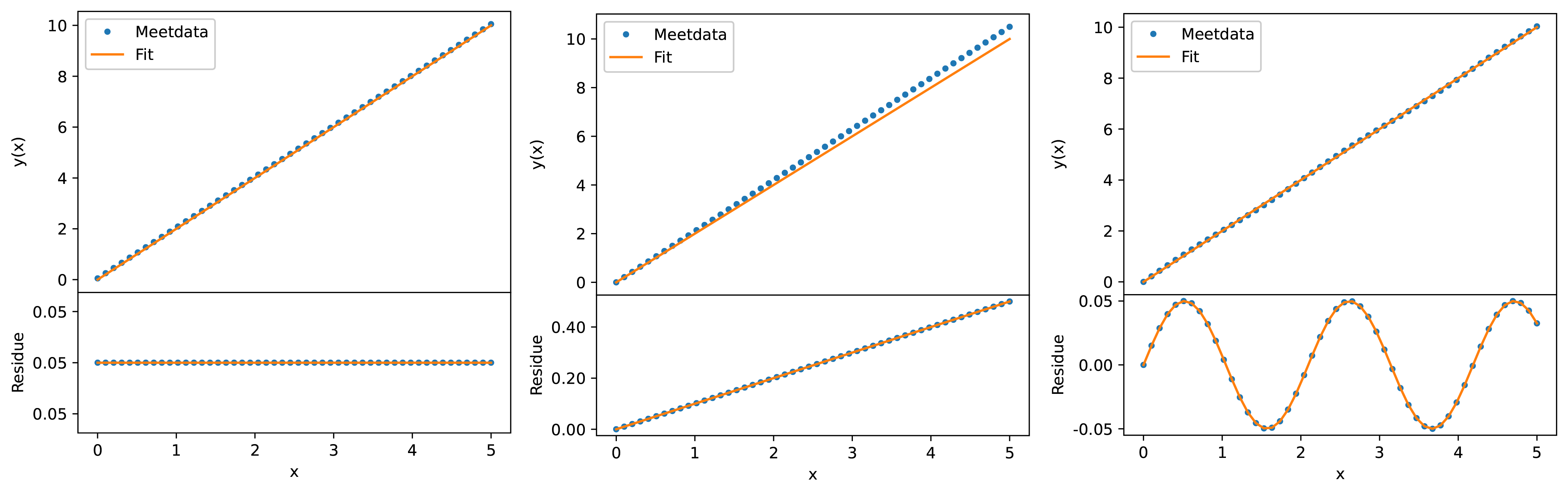
Fig. 24 (a) \(M(x) = 2x + 0.05 \), (b) \(M(x) = 2x + 0.1x\) en \((c) M(x) = 2x + 0.05sin(3x)\). Each measurement contains a ‘hidden’ signal that is visible when analyzing the residuals. In all figures a line \(F(x) = 2x\) was fitted.#
The second analysis of the residue is based on a histogram. If, based on the experiment, you expect the noise to be normally distributed, then the histogram will be a normally distributed function. You can also apply a function fit to this noise signal, whereby we expect the mean to be 0 and the standard deviation to be determinable.
Linearization#
When experimenting, the goal is often to discover the relationship between two variables. In many cases, this relationship is not linear, for example between the swing time and length of a pendulum. In such cases, it is useful to linearize the graphs. Firstly, this makes it easier to see deviations, and secondly, it also makes fitting easier.
Example:
We want to determine the value of the acceleration due to gravity \(g\). To do this, we take measurements between the period \(T\) and the length \(L\) of a pendulum.
According to theory, the relationship between the period and length is as follows: \(T = 2\pi\sqrt{\frac{L}{g}}\) If we square both sides of the equation, we get: \(T^2 = 4\pi^2 \frac{L}{g}.\) By plotting \(T^2\) on the y-axis as a function of \(L\), we have linearized the function, and we can better detect systematic errors.
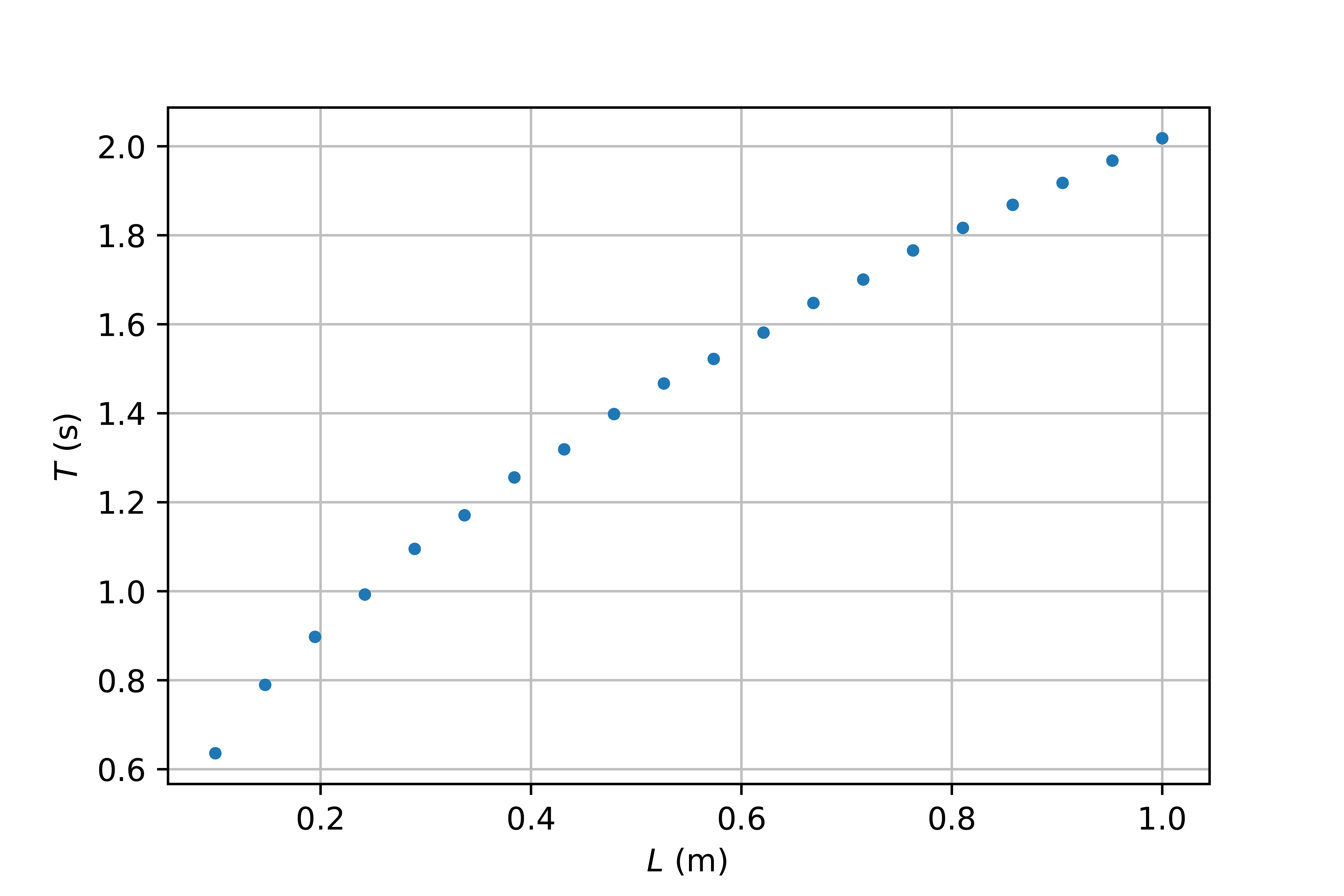
Fig. 25 Measurements of the period as a function of the length. Raw data is plotted, a squared root relation is visible.#
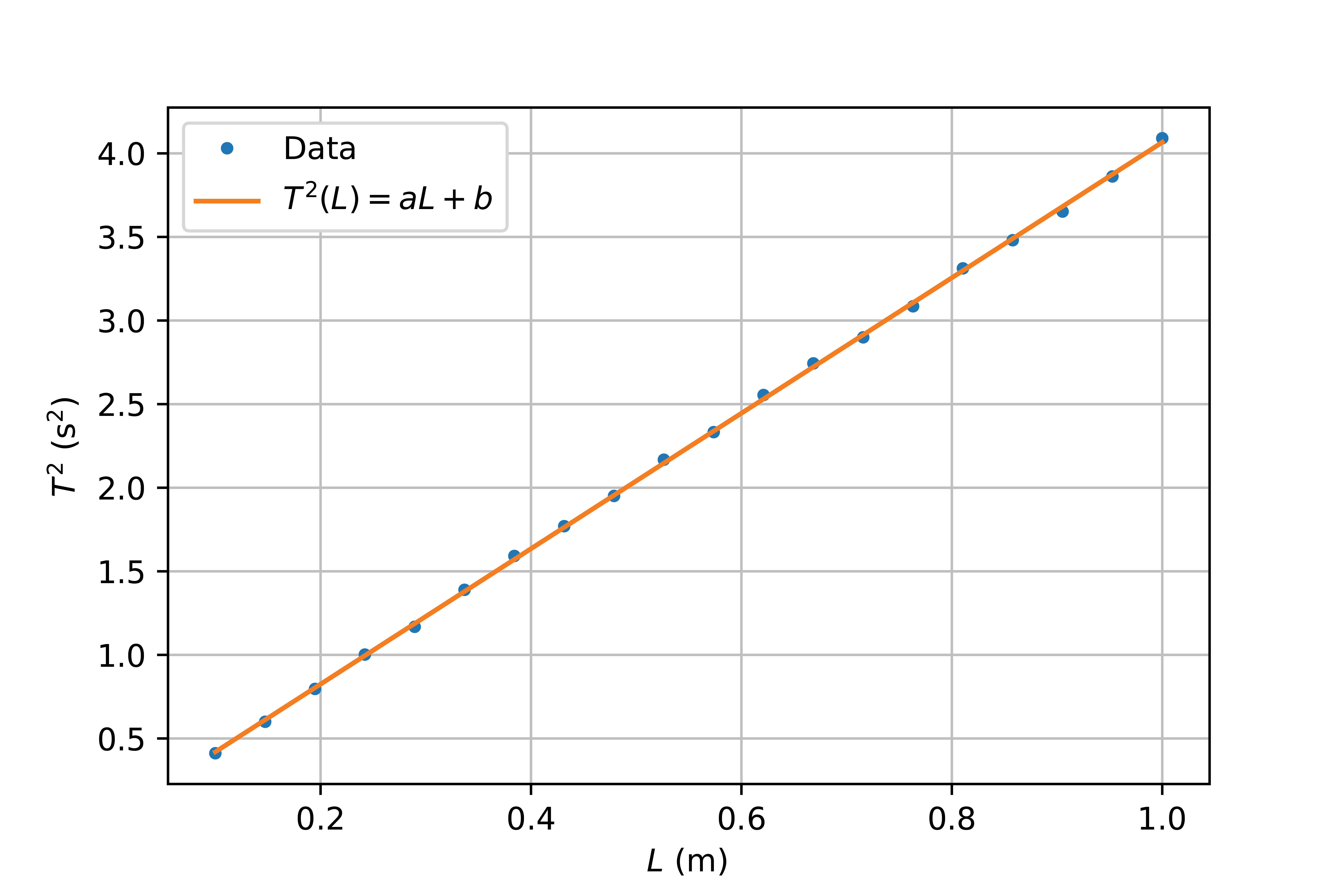
Fig. 26 Linearized data from Figuur 25 by plotting \(T^2\) against \(L\). A first order polynomial \(T^2(L)=aL + b\) was fitted with coefficients \(a = (4.05 \pm0.01)\) s\(^2\)/m and \(b = (0.015 \pm 0.09)\) s\(^2\)#
Agreement analysis#
One of the most important reasons for determining uncertainty is that you want to compare results with each other or with theoretical predictions systematically and quantitatively, and thus determine the extent to which the values differ from each other. The question then is: ‘To what extent do the empirically found values correspond with …’.
Suppose we want to compare two values \(a\) and \(b\), each with their own uncertainty \(u(a)\) and \(u(b)\). Then we first want to look at the difference between these two values: \(v = a- b\). Based on the calculus approach, the uncertainty in \(v\) is given by \(u(v) = \sqrt{u(a)^2 + u(b)^2}\). The agreement now is that two values are inconsistent with each other (in a scientific sense, they do not correspond sufficiently with each other) if the following applies:
When determining physical constants, the uncertainty is often so small that it is negligible compared to other uncertainties. Please note! You could argue that if your measurement uncertainty is large enough, the values will never be contradictory. However, when the uncertainty is relatively large compared to the determined value, the values found have little scientific value.
Great examples of ugly graphs#
There are many ways in which you can present your data poorly. There are only a few ways in which you can do it well. The most important thing when creating a graph is that it is clear and that it is obvious to the reader what they should be looking at.
Figure 27 is a good example of a bad graph. First of all, the trend is not visible. There is one point that is well above the others, but are the values for \(r>11\) equal to 0 or not? In addition, there are far too many numbers (ticks) on the horizontal axis. The scale for the horizontal axis is also poorly chosen. Furthermore, we are missing what is actually presented on the horizontal and vertical axes.
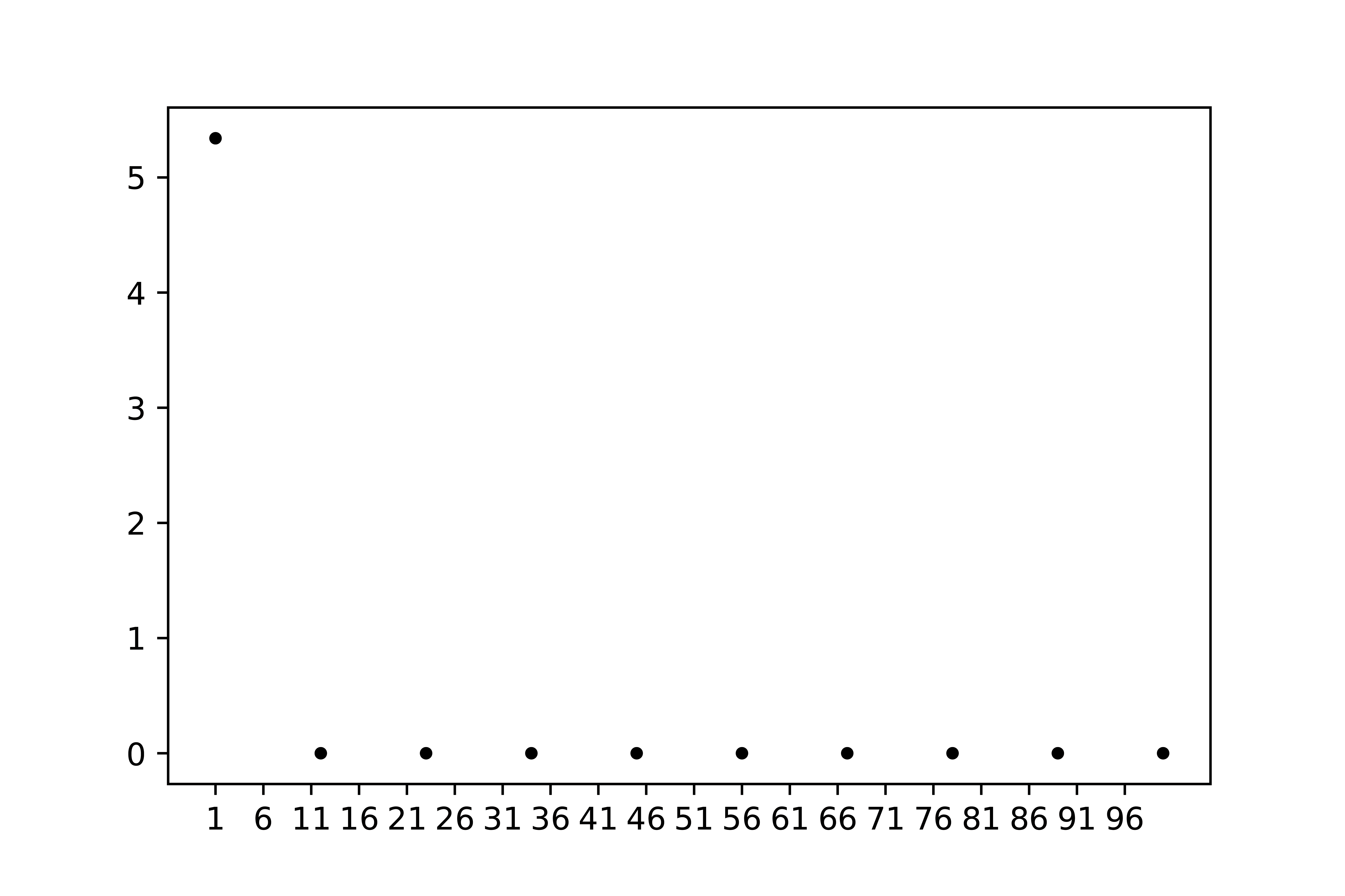
Fig. 27 A great example of an ugly graph#
Figuur 28 presents the same data. The differences may be clear, the data are displayed on a log-log scale, and a trend line shows the relationship between force and distance. The number of ticks is limited. The graph could be further improved by including the measurement uncertainty.
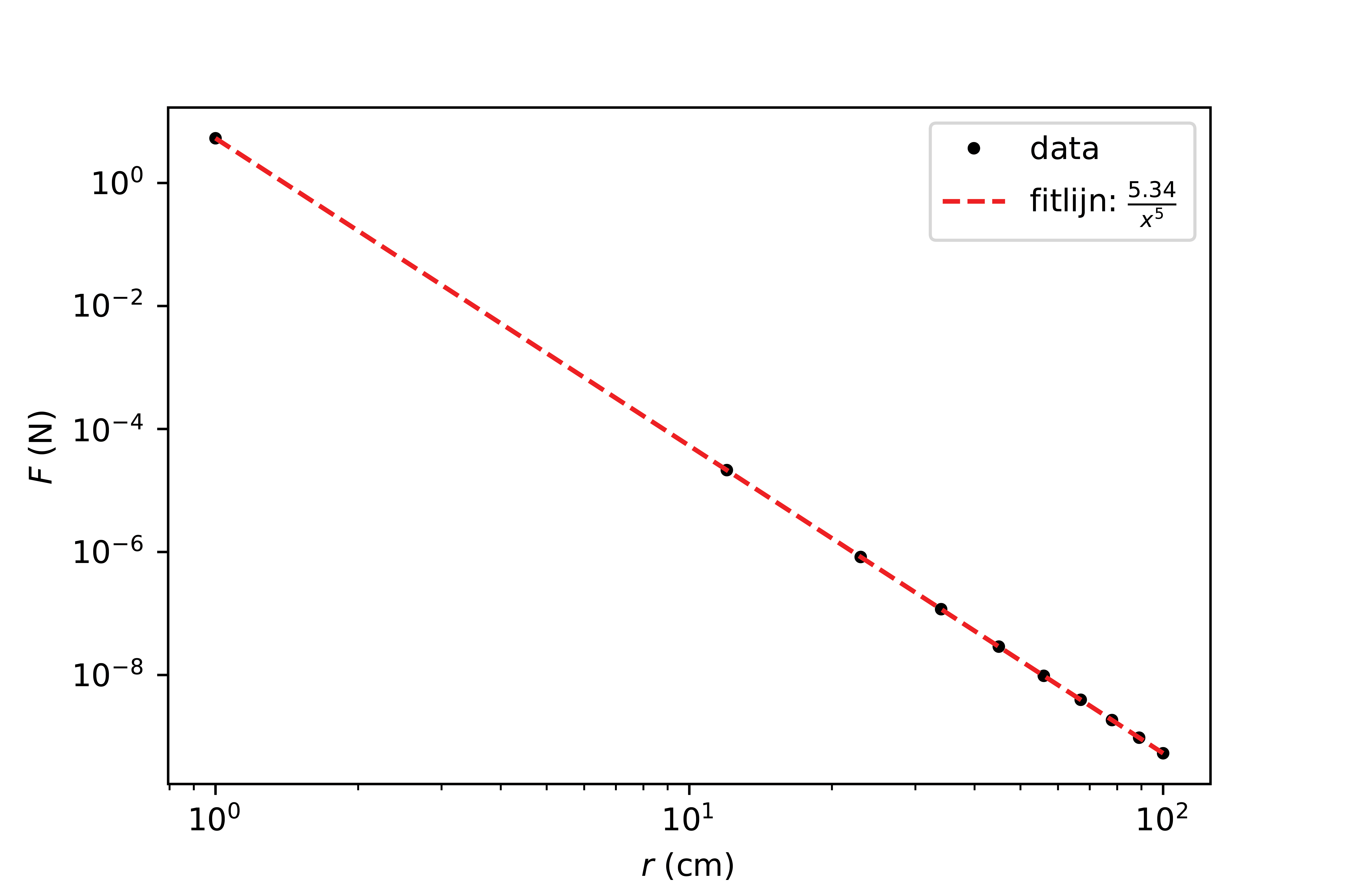
Fig. 28 An improved version of the graph#
Further reading#
Some external sources on the use of data and measurement uncertainty:
Guide to the expression of uncertainty in measurement
Liegen met cijfers
Het bestverkochte boek ooit
Exercises#
Exercise 9
The values of \(a\) and \(x\) are given in the table below.
a |
\(u(a)\) |
x |
\(u(x)\) |
|---|---|---|---|
\(5\cdot10^{-8}\) |
\(1\cdot10^{-9}\) |
\(5\cdot10^{-3}\) |
\(1\cdot10^{-3}\) |
Determine the value and uncertainty of \(F = a \cdot x^{-4}\).
Perform the same exercise as above, but use \(u(a) = 1 \cdot 10^{-9}\) en \(u(x) = 1 \cdot 10^{-10}\). What do you notice?
Keep \(u(a)\) a constant, and use \(u(x) = 1\cdot 10^{-3}\) and \(u(x) = 1\cdot 10^{4}\). What do you notice?
Compare your answers to (2) and (3). Why does the error in \(F\) scale linearly with the error in \(a\), but not with \(x\)?
Solution to Exercise 9
\(F = (5 \pm 6) \cdot 10^1\)
\(F = (50.0 \pm 1.6)\)
Exercise 10
Derive equation (22).
Solution to Exercise 10
First use the calculus method, and then divide by \(f\).
Exercise 11
A distance \(s\) is measured as the difference between two distances \(p\) and \(q\). The positions of \(p\) and \(q\) are: \(p = (30.0\pm0.9)\) km and \(q = (10.0\pm0.1)\) km. Calculate the distance \(s\) and the corresponding uncertainty \(u(s)\). Write the result down using the correct notation.
Solution to Exercise 11
\(s = (20.0 \pm 0.9) \text{km}\)
Exercise 12
Consider a beam with length \(L=(7.5\pm0.1)\) m, width \(B=(12.5\pm0.2)\) cm en height \(H=(15.0\pm0.3)\) cm. The area \(A\) is given by \(B \cdot H\). Determine the uncertainties \(u(A)\) and \(u(V)\).
Solution to Exercise 12
\(u(A) = \sqrt{(\frac{u(B)}{B})}^2+{(\frac{u(H)}{H})^2} \cdot B \cdot H= \sqrt{(\frac{0.2}{12.5})^2+{(\frac{0.3}{15.0})}^2} \cdot 12.5 \cdot 15 = 5 \space \text{cm}^2\)
\(u(V) = \sqrt{{\left(\frac{u(B)}{B}\right)}^2+{\left(\frac{u(H)}{H}\right)}^2+{\left(\frac{u(L)}{L}\right)}^2} \cdot B \cdot H \cdot L= 0.004 \space \text{m}^3\)
Exercise 13
The gravitational acceleration \(g\) is determined using a pendulum. The period is \(T = (1.60\pm0.03)\) s and the length of the pendulum is \(L = (64.0\pm0.8)\) cm.
Give the relation between the period and the length of the pendulum.
Use this relation to derive a formula for the gravitational acceleration \(g\).
Give the formula for the uncertainty \(u(g)\).
Calculate \(g\) and \(u(g)\) and write the results down using the correct notation.
Which variable has the biggest influence of the uncertainty?
Solution to Exercise 13
\(T = 2 \pi \sqrt{\frac{L}{g}}\)
\(g = \frac{4 \pi ^2 L}{T^2}\)
\(\left(\frac{u(g)}{g}\right)^2 = \left(\frac{u(L)}{L}\right)^2 + 4 \left(\frac{u(T)}{T}\right)^2\)
\(g = 9.8696 \space \text{m/s}^2\)
\(u(g) = 0.39 \space \text{m/s}^2\)
dus \(g = (9.9 \space \pm 0.4)\text{m/s}^2\)\(T\), factor 4x as big on the calculation of \(u(g)\). 10x as big in the more precise calculation.
Exercise 14
Variable \(G\) is dependent on the measured variables \(x\) and \(y\), and their relation is \(G(x,y)=\frac{1}{2} x y^{3} + 5 x^{2} y\). The uncertainties in \(x\) and \(y\) are \(u(x)\) and \(u(y)\), respectively. Determine the equation for the uncertainty \(u(G)\).
Solution to Exercise 14
\(G(x,y)=\frac{1}{2} x y^{3} + 5 x^{2} y = G_1 + G_2\)
\(u(G) = \sqrt{u(G_1)^2+u(G_2)^2}\)
\(\left({\frac{u(G_1)}{G_1}}\right)^2 = \left({\frac{u(x)}{x}}\right)^2 + 9 \left({\frac{u(y)}{y}}\right)^2\)
\(\left({\frac{u(G_2)}{G_2}}\right)^2 = 4 \left(\frac{u(x)}{x}\right)^2 + \left({\frac{u(y)}{y}}\right)^2\)
Exercise 15
Consider a sphere with radius \(R=(3.02 \pm 0.06)\) m. Determine the surface area \(A\) and the volume \(V\) with the corresponding (relative) uncertainties.
Solution to Exercise 15
\(A = 4 \pi r ^2 = 114.61 \space \text{m}^2\)
\(u(A) = \sqrt{4 \left(\frac{u(r)}{r}\right)^2} \cdot A = 5 \space \text{m}^2\)
\(A = (115 \pm 5)\) m\(^2\) \(V = \frac{4}{3} \pi r ^3 = 115.37\space \text{m}^3\)
\(u(V) = \sqrt{9 (\frac{u(r)}{r})^2} \cdot V = 7 \space \text{m}^3\)
\(V = (115 \pm 7)\space \text{m}^3\)
Exercise 16
Consider \(f(x)=2\sin{x}\), with \(x\) a measured quantity with uncertainty \(u(x)\). Derive an equation for the uncertainty \(u(f)\).
Solution to Exercise 16
\(u(f) = |\frac{\partial f}{\partial x}| \cdot u(x) = |\frac{\partial 2\sin(x)}{\partial x}| \cdot u(x) = 2|\cos(x)| \cdot u(x)\)
Exercise 17
How can you linearize the relations (1-4) below, such that they can be plotted as a straight line \(y = mx + c\)? Give the expression for the slope \(m\), and the intersection \(c\).
\(V = aU^2\)
\(V = a\sqrt{U}\)
\(V = a \exp{(-bU)}\)
\(\frac{1}{U} + \frac{1}{V} = \frac{1}{a}\)
Solution to Exercise 17
\(y\)-axis: \(\sqrt{V}\), \(x\)-axis: \(U\). m: \(\sqrt{a}\), c: 0
\(y\)-axis: \(V^2\), \(x\)-axis: \(U\). m: \(a^2\), c: 0
\(y\)-axis: \(\ln{V}\), \(x\)-axis: \(U\). m: \(-b\), c: 0
\(y\)-axis: \(\frac{1}{V}\), \(x\)-axis: \(\frac{1}{U}\). m: \(-1\), c: \(\frac{1}{a}\)
\(\frac{1}{U} + \frac{1}{V} = \frac{1}{a}\)