Goal
This experiment consists of two parts. The goal of these experiments are to get acquainted with electronics and electronic instruments. These instruments are often used in more advanced physics labs.
Part 1: Boltzmann constant
The goal of the experiment is to gain experience with Digital Multi Meters (DMMs) with an experiment in which you determine the Boltzmann constant. We use a frequently used setup, the ‘‘voltage divider’’.
This video is a great introduction to this experiment.
Background
Measurements using DMMs
DMMs are versatile measuring instruments. These instruments are used to measure voltage, current, resistance, frequencies, periods, capacities, induction, temperature, features of diodes etc. Advanced DMMs have the option to be controlled using a computer.
The difference in price is often determined by its functionality, resolution and sensitivity. The resolution of a digital instrument is the ratio between the smallest counts and the largest counts that can be displayed. This is determined by the number of counts that can be displayed. A simple DMM often has digits, which means that the DMM can display three whole digits (0-9) and an additional (first) digit which has the value 0 or ± 1. As such, this DMM can display the number 0-1999, a total of 2000 counts. The resolution of this DMM is thus or 0.05%.
The sensitivity is the smallest change that still can be noted. A sensitivity of implies that signals smaller than can not be detected. The sensitivity does depend on the amplitude of the signal we want to measure. Suppose we want to measure a signal using a DMM, the best range is . This means a sensitivity of . Using a DMM, we can get a sensitivity of . The ultimate sensitivity of a DMM depends on the resolution and the smallest range. Example: the sensitivity of a digit DMM with the smallest range of is .
However, measuring does not mean this is the exact value you measure. This does depend on the accuracy, and the accuracy is not determined by the last digit of the DMM alone. The accuracy is often defined as ‘’..% reading + ..%range + .. counts’'.
Example
Suppose we use a digit DMM and read a value of . For the Dynatek D9100 with a range is stated that the inaccuracy is given by: of the reading + 1 count. So: 0.5% of the reading yields + 1 digit () gives an accuracy of . The reading should be written as: .
The accuracy of a DMM in the range of is defined as: 0.0015% of the reading and 0.0004% of the range. The reading on the DMM is . What is the accuracy of the measurement?
What is the sensitivity of a measurement using a digit DMM with a range?
Ideal instruments
A DMM can be used as a voltmeter or ammeter. In the ideal case a voltmeter has an infinite internal resistance and an ammeter no resistance. In many cases these assumptions are valid. However, in cases where the circuit resistance is approximately 0 or , we can not neglect the features of the meters. Using these meters inevitably changes the features of the circuits itself, see Figure 2.
Figure 2 shows two circuits in which the current through and voltage over a diode is measured.
Which circuit do you use when the resistance of the diode is very small? Explain why.
Which circuit do you use when the resistance of the diode is very large? Explain why.
How does the resistor prevent blowing up the fuse of the Ammeter?
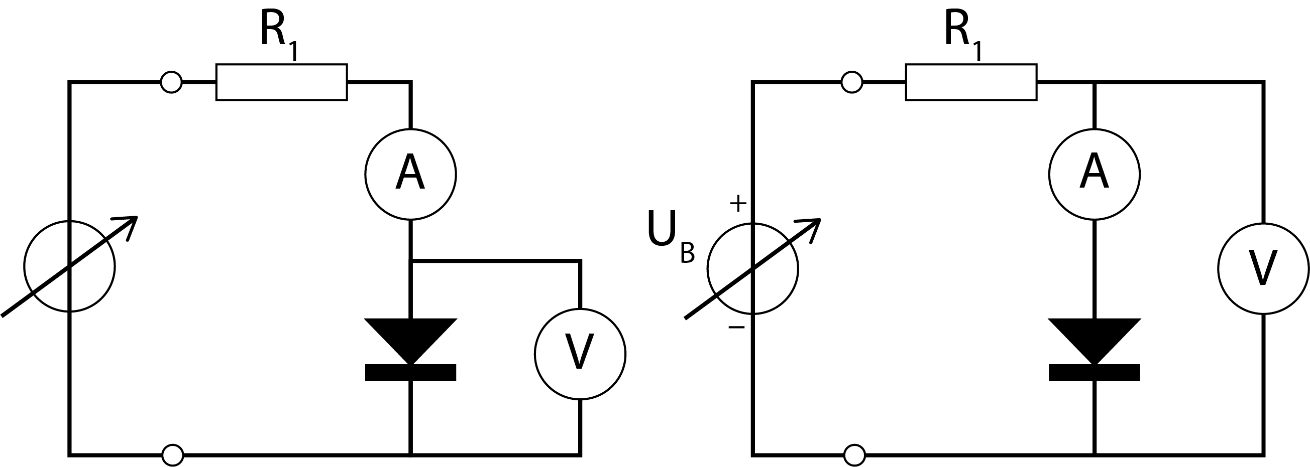
Figure 2:Two ways of measuring current and voltage through a diode
In this experiment we will determine the -characteristics of a silicon diode. However, during the experiment the current through the diode easily changes with 6 decades (). Therefore we measure the current indirectly, using a voltage divider.
Voltage divider
In this experiment we use a voltage divider circuit to make a -characteristic of a diode, see Figure 3. A simple voltage divider is a circuit with two resistors in series ‘‘sharing’’ the voltage of the source. If you do not remember the rules that apply in series circuits, look these up yourselves. The formulas are given below.
An advantages of this circuit is that we do not measure current directly. As the current changes a few decades, we approximate the original circuit (without instruments).
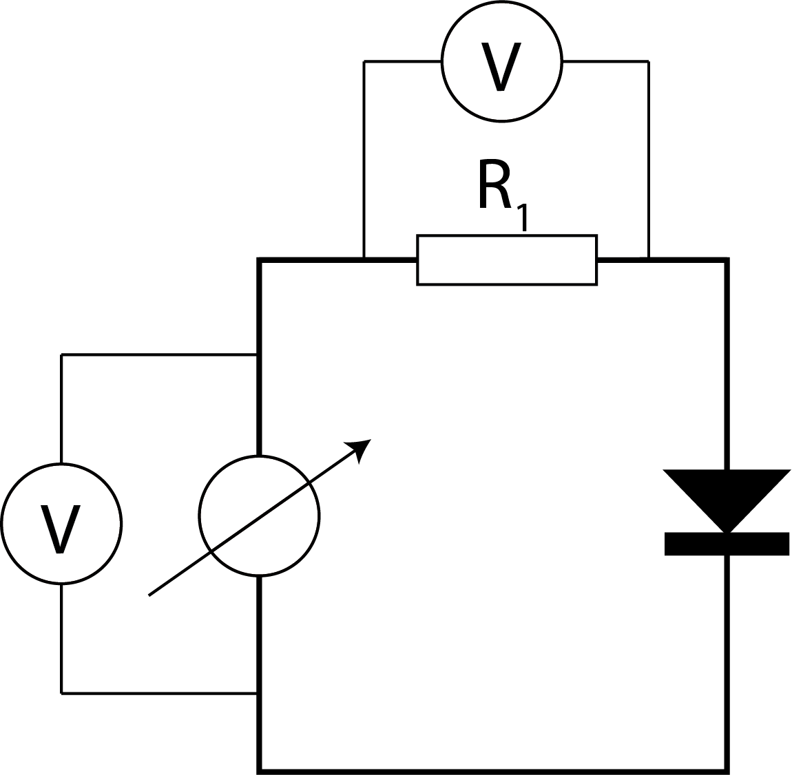
Figure 3:The experimental setup to determine the -characteristic of the diode
Explain how you will obtain the current running through the diode using circuit Figure 3.
Suppose we have a voltage divider consisting a and a resistor.
Calculate the maximum current through the resistor if the maximum dissipation in the resistors is .
What is the maximum source voltage which can be applied such that the maximum permissible dissipation is not exceeded?
Calculate the voltage over the resistor if the source voltage is .
A voltage divider is used as a sensor for an automatic night lamp. It circuit consist of an Ohmic resistor and a light dependent resistor (LDR) in series. The LDR has a resistance of about in the dark and a resistance of about in the light. The sensor works best when a small change in the resistance of the LDR changes the voltage of the Ohmic resistor as much as possible.
What value should the Ohmic resistor ideally have? [hint: Physicist often use extreme cases to calculate what happens (0,,R)].
In our experiment the diode has a resistance of more than . Why is it not wise to choose ?
Semiconductor diode
A diode is a semiconductor. In a semiconductor the energy of the electrons are distributed according the Boltzmann distribution. The average energy of an electron is , where is the Boltzmann constant and is the absolute temperature. The current flowing through the circuit depends on the height of the energy barrier relative to . On its turn, the height of the barrier depends on the the applied voltage. The higher the applied voltage the lower the energy barrier.
The Boltzmann distribution of the energy of the electrons, and the presence of a barrier is given by a theoretical formula that relates the applied voltage over and the current through a diode. This is an exponential function given by:
where is the charge of an electron, , an ideality factor which is 2 for Si, the reverse current when is strongly negative. For more (background) information, refer to Wolfson & others (2007), chapter 27-28.
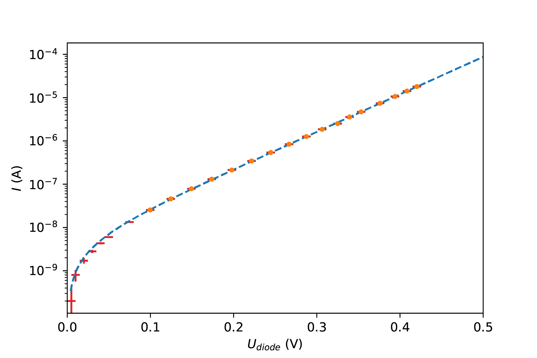
Figure 4:The -characteristic of the diode as determined by two first year physics students (2019). The slope is used to determine the Boltzmann constant.
In order to enable us to determine the -characteristics of a silicon diode (over a range which is as large as possible), we should consider a number of topics before we actually conduct the experiment. We note that we aim to determine Boltzmann’s constant using a logarithmic plot. To do this accurately, it is key to distribute measurements evenly along the range of the variables (diode current and diode voltage ). In practice, it is convenient to start at (or near) the maximum value for the current and subsequently decrease the current with a constant factor for each measurement. However, it might be simpler to measure, plot and choose the next value based upon your findings.
Method
Preparation phase
Prepare you python script in which you collect and process your data. Carry out the following steps:
Load the various libraries. (single cell)
Make numpy arrays for your raw measurements. (single cell)
Make numpy arrays for the processed data and their uncertainties. Use the manual of the DMM to calculate the uncertainties. (single cell)
Make a single cell in which you plot the -characteristics of the diode.
Setup a single cell for curve fitting.
Setup a single cell for calculating the Boltzmann constant and its uncertainty.
Experimental phase
Determine the exact resistance of the resistors you will use, calculate the uncertainty. Build the circuit shown in Figure 3. Start your measurements with a source voltage. Slowly decrease the source voltage using the plot. Make sure you have at least 15 measurements in the range for . Take care of an even spread interval.
Evaluation phase
Run your script and determine the Boltzmann constant accordingly. You should be at least within 5% accuracy.
Part 2 As function of temperature
https://
In the experiment described above it is possible investigated the characteristic of a diode at a constant temperature. However, the Boltzmann energy distribution also includes a temperature dependence. Based on this experiment, the effect of temperature on the characteristic of a diode and an Ohmic resistor can be determined.
Introduction
Both the classical free-electron model and the quantum mechanical free-electron model lead to Ohmic behavior for the conduction of metals and semiconductors. In this experiment, the resistance is measured as a function of temperature for a metal (which satisfies the criteria of a free electron gas) and two semiconductors. By the end of the project, you are expected to interpret the measurement results according to the microscopic conduction model, where the concepts of electron mass, electron density, electron charge, and relaxation- (or collision-) time are addressed, along with the influence of temperature on these quantities. The conduction models must be verified or falsified through interpretation.
In the microscopic picture of electrical conduction, Ohm’s law results in a relationship (eq 38.12, page 1235 Tipler & Mosca (2007)) between the specific resistance () and the effective electron mass (), charge carrier density (), elementary charge (), and the time between two successive collisions ():
In a metal, the electron density does not strongly depend on temperature , but the time between two successive collisions () is crucial for conduction.
Classical conduction theory predicts a temperature dependence proportional to the square root of the temperature ().
The kinetic energy of the electron is given by three degrees of freedom (i.e., movements in the x, y, and z directions), each contributing to the total energy (equipartition theorem, p 544 Tipler & Mosca (2007)):
where is the velocity of the electron, and is the Boltzmann constant.
In the quantum mechanical model, lattice vibrations primarily limit the collision time. Because the number of quantized lattice vibrations increases linearly with temperature at low temperatures, the collision time and therefore the specific resistance also increase linearly with temperature.
For conduction in semiconductors, temperature changes in collision time are much smaller than changes in charge carrier density. Due to the forbidden band gap, the occupied valence bands and unoccupied conduction bands are separated. Conduction occurs through electrons in the conduction band and holes in the valence band. The probability that a valence electron can be thermally excited from the valence band to the conduction band is given by the Fermi-Dirac distribution (eq 38.45, p 1257 Tipler & Mosca (2007)):
where is the electron’s energy, and represents the bandgap energy.
Equipment
Cryostat
Temperature-dependent measurements are usually performed in a cryostat. This device consists of several compartments. The innermost compartment is the sample space, where the sample to be measured is located, optionally with a small oven for heating. Surrounding the sample space is a compartment for the coolant (liquid nitrogen or helium). In this experiment, liquid nitrogen is used for cooling. Nitrogen has a boiling point of at an atmospheric pressure of .
Between the space for the liquid nitrogen and the outer wall, there is an insulation compartment that is under vacuum, so that no heat is transferred to the liquid nitrogen through convection. Additionally, there is an absorption pump in this space that starts pumping once the compartment for the coolant is filled. The surfaces in this insulation space that face outward are also provided with a layer of super insulation that has a high reflective ability for thermal radiation.
One or more samples can be attached to the sample rod in an IC socket. A heating tape wrapped around the sample holder acts as a small oven to set the temperature from the boiling point of liquid nitrogen to . A thermocouple sensor weld is also attached to the sample rod, which records the temperature of the sample holder.
Thermocouple
The temperature is measured using a thermocouple and a readout unit. This unit measures the thermoelectric voltage of the measuring junction (a metal/metal contact) and displays the temperature in degrees Celsius on the screen. The voltage of the reference junction is automatically compensated. The reference table for a copper/constantan (type T) thermocouple is stored in the memory of this unit. With a type T thermocouple, the temperature can be reliably measured in the range from to .
Power Supply and DMM
A power supply is available to drive the heating tape. The inventory of this experiment includes three digital multimeters to measure the resistance of the choke coil and the operating points of the diode.
Tasks
The quantum mechanical free electron model How is the temperature dependence expressed in this model? Sketch the expected behavior of the specific resistance as a function of temperature for a metal.
DC current in a diode is determined by the probability that the electrons can make the potential step from n p. The current in a diode is therefore given by:
Here, is the dark current, which is determined by the probability that electrons are thermally excited from the valence band to the conduction band:
From (9) and (10), it follows that:
For a constant current , the voltage across a diode in the forward direction is linear with temperature.
Sketch the voltage behavior as a function of temperature and indicate how the bandgap can be determined from this.
Tip
In the original experiment, the resistance of the choke coil and diodes in the cryostat had to be measured in the temperature range from to with steps of , and heated at a rate of 2 degrees per minute.
- Wolfson, R., & others. (2007). Essential university physics (Vol. 1). Addison-Wesley San Francisco, CA.
- Tipler, P. A., & Mosca, G. (2007). Physics for Scientists and Engineers (6th ed.). W. H. Freeman.