Goal
In the first part of this experiment you will determine the half-life of the naturally occurring radioactive atomic species , an isotope of the element potassium. You will do this by establishing of the activity and the number of radioactive nuclei of samples. In the second part you will establish a histogram of the number of measured decay processes and you will fit a Poisson probability function to the histogram. The fit will also yield a value of the half-life of , which should be compared with the value resulting from the first part. The question is which method yields the best result and whether there is a trade-off.
Introduction
The natural background of ionizing radiation
Although not generally known, everyone is exposed to ionizing radiation of natural origin. This radiation originates from both cosmic and terrestrial sources. Terrestrial radiation arises from several kinds of radioactive substances. Some of these substances are present because of human activity (nuclear tests, nuclear power plants). A substantial part of these substances, however, occurs naturally and comprises radioactive nuclides with a long lifetime. This category includes uranium isotopes and the radioactive decay products of these isotopes, including the noble gas radon. The natural composition of potassium also includes and isotope with a very long lifetime: .
This potassium isotope dominantly decays to by emission of an electron, so-called -decay. Further processes are -decay (emission of a positron, i.e. a positively charged electron) or capture of an electron from an electron shell close to the nucleus (electron capture, EC). In these cases the decay product is . A decay scheme of is given in Figure 1 U.S. Department of Health, Education, and Welfare (1970).
The lifetime of must be of the same order of magnitude as that of the lifetime of the Earth. Otherwise, the formed in creation of the Earth would have disappeared already by radioactive decay.
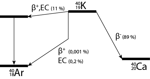
Figure 1:Decay scheme of . Vertical lines correspond to emission of gamma radiation. EC: electron capture.
Equivalent dose from background radiation
In expressing the potential risks due to radiation the equivalent dose is often used. This is the radiation load due to ionizing radiation. The equivalent dose is the absorbed dose (absorbed energy per kg material) multiplied by a factor representing the biological effectiveness of the radiation. The SI unit of equivalent dose is the Sievert ().
In the Netherlands, the equivalent dose resulting from natural sources is roughly per year of which roughly 10% is due to the decay of . In comparison, having an X-ray in a hospital also gives an equivalent dose of several tenths of mSv. A skiing holiday or a transatlantic flight, since one is higher up in the atmosphere, give equivalent doses of one hundredth to one tenth of a .
Theory of the radioactive decay
Average behaviour
Suppose we have a number of nuclei of a radioactive nuclide at time . It is reasonable to assume that the number of nuclei that decays () on average in a time span is both proportional to and :
Here, the proportionality factor is called the decay constant. Equation (1) is in fact a differential equation for . Its solution,the law of radioactive decay, is an exponentially decaying function in time:
The inverse of , i.e. , is called the average lifetime of the nuclide. This is the time it takes for the number of parent nuclei to decrease to 1/e of its initial value. Additionally, the half-life is often used. This is the time it takes for half the original nuclei to decay. By substituting in Eq. (2) the value for , it easily follows that
The decay constant (and hence the average lifetime and the half-life) is a characteristic of a radioactive nuclide, for example . The activity of a radioactive source is the number of nuclei that decay per unit of time:
The activity also decays exponentially in time, again with constant . The activity has the dimension and thus can be expressed in . However, there is a distinct SI-unit for activity of a radioactive source, the becquerel (). In this context, we note that a count rate should be expressed in the unit in or a similar unit (e.g. ). A count rate only becomes an activity with unit after correction for a number of effects, such as background radiation and the efficiency of the setup.
Statistics of the decay
Equation (2) describes the average behaviour of radioactive decay. On a short time scale, however, the decay has a random character. The number of decay processes taking place in a time interval t varies in time and shows a statistical behaviour around the mean . The statistical probability that k nuclei of the nuclei present in the sample decay in the time interval is given by the Poisson probability distribution :
The parameter is the mean number of decay processes in a time interval . The value of can be calculated from the values of k measured for a very large number of in-dependent time intervals (of equal size). The function k! (pronounce: k faculty) is the factorial function given by (with 0!=1).
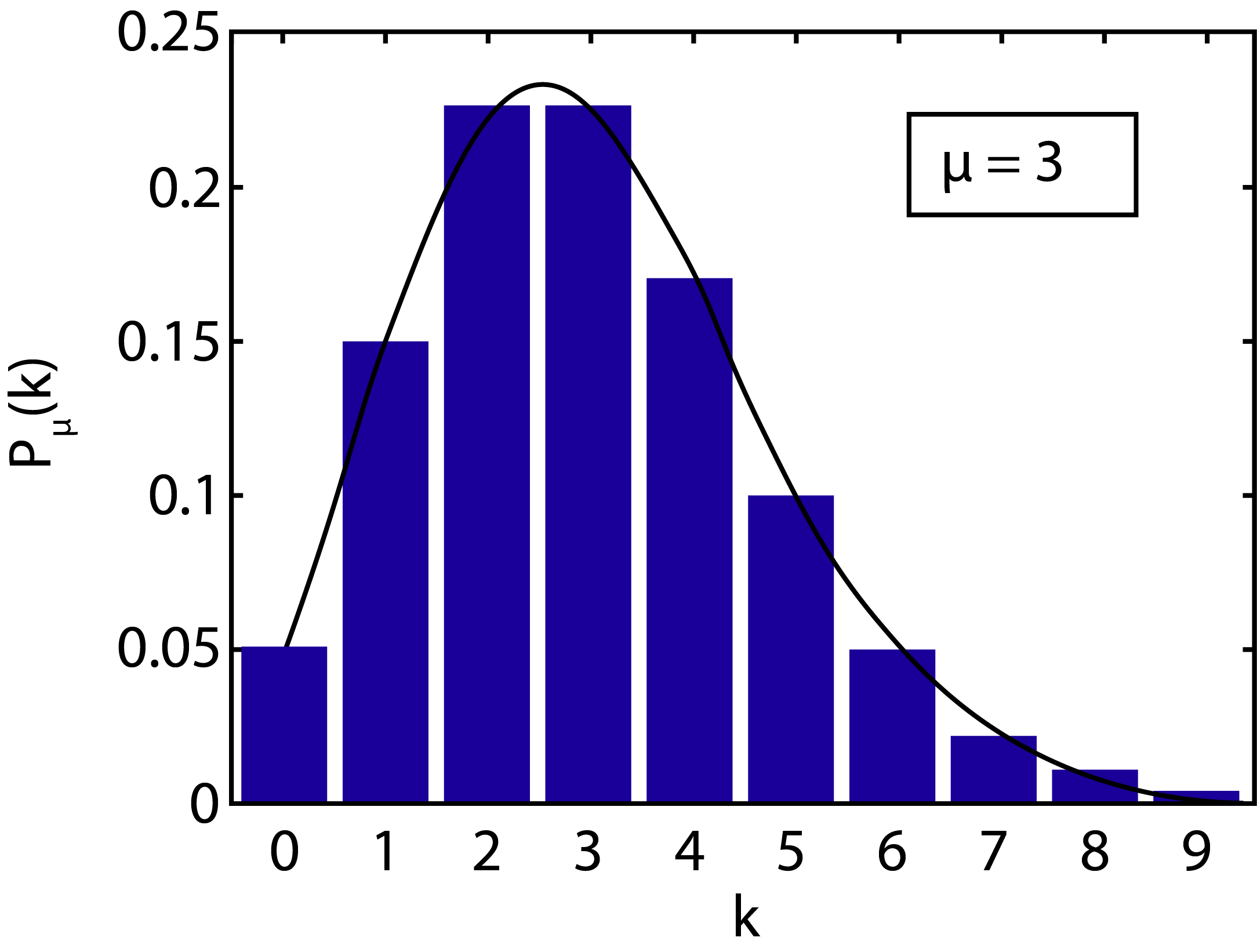
Figure 2:Poisson probability distribution for , plotted together with the histogram to which the distribution has been fitted. The probability distribution is asymmetric. The curve has been plotted as a continuous curve, but in reality the distribution only holds for integer values of k.
Although Eq. (5) gives a relatively simple function, it is difficult to remember how and k are placed in the expression (Advice: keep on paying attention to this!). From Eq. (5) it follows that the Poisson probability distribution is determined by only a single parameter , the mean of the distribution. Figure 2 shows the plot of a Poisson distribution for . It can be noticed immediately that the Poisson distribution is not symmetric, a property most easily seen for .
An expression for based on the average behaviour of the radioactive decay can be obtained by multiplying the average decrease of the number of radioactive nuclei per unit of time [i.e. the activity, Eq. (4)] with the time interval :
Omitting the time dependence of N in the last part of this equation indicates that the number of radioactive nuclei only decreases negligibly in the time interval . (N.b.: usually, the notation for a time interval is ; generally, t denotes a point in time.)
Typically, in measuring radioactive decay, a counting experiment is performed. In such an experiment the number of decay processes in the time interval is counted by detection of the decay products. By repeating the counting many times and making a histogram of the count totals in the time intervals , a distribution is obtained. This distribution will confirm the Poisson distribution. Apart from the mean, the standard deviation is an important characteristic of the Poisson distribution. In particular, determines the width of the distribution. From the definition of the standard deviation and Eq. (5), one can derive:
Thus, the parameter is not only the mean of the distribution, but also determines its standard deviation. Equation (7) is often generalised to the square root rule for an individual counting experiment (not limited to radioactive decay; for example the number of babies born per month in a hospital): the uncertainty in a counting experiment with a count total of k is . The fractional uncertainty then is
implying it pays off to score a higher count total, for instance by using a source of higher activity or by measuring during a longer time period.
We now address two more topics about the Poisson distribution: the normalisation of the distribution and the calculation of the mean using Eq. (5).
Normalisation: For a probability distribution the sum of all probabilities equals unity. This applies to the Poison distribution as well:
The correctness of Eq. (9) immediately follows from the Taylor series expansion of
Calculation of the mean: the property that is the mean number of decay processes can be proven by summing over all possible value of k, each multiplied by the probability of its occurrence:
The Poisson distribution typically holds for a probability experiment with a very large population and a small probability of success. Here, success means that a nucleus decays; in Eq. (5) counts the number of successes. For radioactive decay the population is the very large number of radioactive nuclei (here: ), while the probability of success is given by the small number (here: ). In the terminology of statistics, each individual counting experiment during a time period can be seen as attempts (since there are nuclei). In each counting experiment, the count is made how many of attempts lead to success.
In the limit of very large , the asymmetric Poisson distribution turns into the symmetric normal distribution, which in general is determined by two independent parameters (the mean and the standard deviation). For rare and random decay processes, however, only the parameter of the original Poisson distribution determines the resulting normal distribution (again with: mean = and standard deviation = ).
Determination of the Half-Life of 
From the preceding chapter it follows that the half-life of a nuclide can be determined by measuring the activity as a function of time. One could measure the count rate and, if needed, correct it for background radiation. The corrected count rate is proportional to the activity. If the corrected count rate is plotted on a logarithmic scale versus time, then within the measurement uncertainty a straight line results with a slope , from which can be calculated using Eq. (3).
However, a sample containing is not expected to show a decrease of activity during any realistic measurement time, given the half-life of billions of years. Therefore, our first method to obtain the half-life is based on Eq. (4), by determining and . Indeed, according to Eq. (4) we have
And from Eq. (3) it follows
The other way of determining is by experimentally obtaining the histogram of count totals, each total measured during the time interval . By fitting a Poisson distribution to the histogram the mean is obtained, which via Eq. (6) leads to .
Determining the number of nuclei in one gram of KCl
The quantities and in the equation for the half-life relate to the same number of nuclei. This situation can be realized by reducing measurement results from different samples to the mass of one gram of . When we redefine as the number of nuclei in one gram of , then can be expressed in , and . is the fraction of the presence (abundance) of the isotope in the natural isotope mixture, is the Avogadro constant, is the molar mass of . The values of , and can be looked up in a data compendium, for example James & Lord (1992).
Determining the activity of one gram of KCl
To determine the activity of one gram of , we use the setup depicted in Figure 3. The heart of the setup is a Geiger-Muller (GM) detector, applied in this experiment to detect electrons.
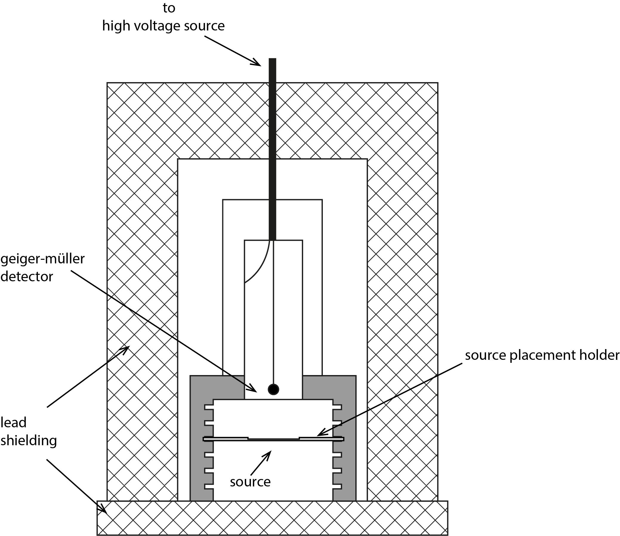
Figure 3:Geiger-Muller counting setup for determining the half-live of . Sample holders are available to accommodate different thicknesses of KCl powder. The holder should be placed in the uppermost slot.
Typically, the number of detections induced by the sample is counted during a certain time period, using a counter/timer. The count rate R is obtained by dividing the count total by the measurement time . Since the count rate is not equal to the activity, it is therefore expressed in and not in . The count rate is recalculated into the activity by making several corrections. The discussion below is limited to those corrections that give a significant contribution.
1. Background radiation
The count rate should be corrected for the background radiation. To determine the background, a count is made without the sample in place. The count is taken over a time period as long as reasonably possible, to minimize the relative uncertainty of the correction. The resulting count rate corrected for the background then is
where is the count total for the background and the duration of background counting. From the count rate per gram is given by
with the mass of the sample in grams.
2. Efficiency
Since not each decay induces a detection, further correction of the count rate is needed. The ratio of the count rate to the activity is called the efficiency. The total efficiency is determined by three factors: (a) the self-absorption in the source, (b) the -efficiency of the GM detector and (c) the geometric efficiency of the setup.
a. Self-absorption.
With increasing sample thickness, more decay products will be absorbed in the source itself and will thus not reach the detector. This effect of self-absorption can be corrected for by measuring the rate as a function of sample thickness and by extrapolating the results to zero thickness. To enable this, sample holders are available to accommodate different thicknesses of powder. The extrapolation including uncertainty analysis is performed in Python, using a least squares fit of a polynomial to the data points and taking into account the error bars of the points. When using a polynomial, the following relation between and is assumed to hold:
The least squares fit yields the coefficients of the polynomial. Extrapolation to zero thickness implies setting in the fitted polynomial, thus obtaining . Thus, is the self-absorption corrected count rate of 1 gram of , obtained via determining the count rate per gram as a function of sample thickness including correction for the background. In the symbol the index “corr” denotes correction for the background, while the index “0” denotes extrapolation to zero sample thickness.
b. The -efficiency:
This is the ratio of the number of detected -particles to the number of -particles reaching the GM-tube. The value of is given in the data sheet of the setup.
c. Geometric efficiency: G
This is the ratio of the number of electrons reaching the detector to the number of electrons that are emitted by the source. Since electron emission from the source is omnidirectional and the detector does not completely enclose the source, only a fraction of the electrons will reach the detector. This geometric efficiency relates to the solid angle under which the detector “sees” the source (solid angle is the three-dimensional equivalent of angle in the plane). For a point source the solid angle can be easily calculated. In our case, however, the source is not a point source, resulting in a rather complex expression for G:
Here and , with s the distance between the source and the detector window, the radius of the circular and flat detector window and the radius of the circular and flat source (see Figure 4).
You can verify that:
Equation (16) is rather complex, making the complete uncertainty analysis for the efficiency rather involved. Therefore, the value of and the corresponding uncertainty are given here: , with .
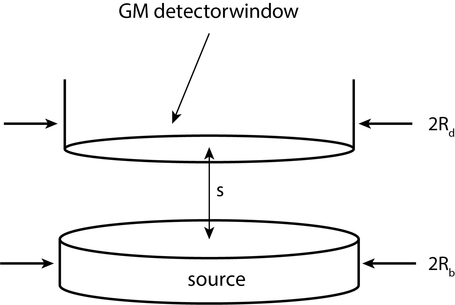
Figure 4:Geometry of the source and detector, with indication of relevant dimensions.
3. Fraction of -decay
The last correction to be discussed relates to the property of the GM detector of only detecting the -decay. The very few positrons emitted in the -decay (see Figure 1) annihilate with electrons of the and ions and thus will not reach the detector. This positron annihilation results in -radiation, for which the detector has a very low efficiency. Electron capture (EC, see Figure 1) will mainly result in X-ray photons, of which a very high fraction is absorbed in the source. It follows that of the three decay channels only the fraction of -decay is seen by the detector. This fraction is denoted by the symbol .
Assignments
For the formulation of the problem, see the chapter GOAL. A separate afternoon will be scheduled to work on the problem analysis aad a measurement plan. For data processing and data plotting you will use Python. In particular, you will use Python for making least squares fits of functions (polynomial and Poisson distribution) to the experimental data.
Part 1: Determining the half-life from the activity and the number of nuclei
Before equation (12) can be applied to determine the half-life, the number of nuclei and the measured activity , both per gram, should be expressed. These can be calculated from the measuring data or taken from literature. The related assignments are:
Express in , and .
Look up the values for , and , including their uncertainties, and write these down.
Write as a function of the quantities , , and . You will calculate the value of in assignment 9 below, the three other quantities can be looked up.
Look up the values for , and , including their uncertainties, and write these down.
Write the half-life as a function of the quantities , , , , , and using Eq. (12) and the expressions derived for and
Derive the equation for the relative uncertainty of using the expression for just obtained. Determine those contributions to the total uncertainty that can be neglected.
Study the measurement setup. The sample holders should be placed in the upper-most slot, since the G-value given in paragraph 4.2 holds for this position.
The raw count data, measured as a function of sample thickness, must be converted to count rates . Based on Eqs. (13) and (14), write as a function of quantities that either can be measured directly or can be set to a certain value.
To determine , make a plot in Python of as a function of and extrapolate the polynomial fit to . Include the error bars for the data points in your plot, for which you will need the uncertainty of . Derive the expression for the uncertainty of and determine which contributions can be neglected.
What is the literature value of the half-life of in literature?
Part 2: Determining the half-life from the Poisson distribution
You will repeatedly count the number of decayed nuclei during a time interval and determine the Poisson distribution corresponding to the count totals. The resulting fit parameter is , which is related to the half-life according to Eq. (6). Assignments:
To obtain an accurate approximation of the Poisson distribution, you have to perform at least 200 individual counts. Choose the time interval such that the average number of counts in the interval is less than 10. Choose the sample holder with the most shallow cavity (why?) and again use the uppermost slot.
Determine the mean from the count totals, using Python. This will be your first estimate of . A logical way for this is by putting the count totals in a vector . Additionally, use:
min(N)
max(N)
len(N)
mu = sum(N)/len(N)
With Python, plot a histogram of the count totals. Then add the Poisson distribution for the value of (from assignment 12) to the same plot. For the plot you may approximate the Poisson distribution by replacing in Eq. (5) with the gamma function for the argument . By doing so, can also be calculated for non-integer values of . Don’t forget to add to the top of the script:
from scipy.special import gammaFor calculating and plotting a histogram, with 25 bins, with the centers corresponding to the number of counts within (here 0 to 24), the input in Python will be
n = plt.hist(N, bins=25, range=[-0.5, 24.5], rwidth=0.9)We like to add the theoretical distribution corresponding to the value of of Assignment 12 to the plot. To this end prepare an array with closely spaced values
kf. For instance:kf = np.linspace(-0.5,24.5,100) Pois = len(N)*(mu**kf)*np.exp(-mu)/gamma(kf+1) plt.plot(kf,Pois,color='k', linestyle='dashed')
If needed, you can adapt the axes: range, labels, font size.
Then, use
curve_fitto fit the frequencies (= the number in the bins) to the Poisson distribution. The fit function is:def func(x,a): y = len(N)*(a**x)*exp(-a)/gamma(x+1) return yNOTE: It’s not possible to directly multiply
func()in the argument ofcurve_fitwithlen(N). Therefore, we have to incorporatelen(N)in the function definition. You could fit this as a parameter as well, but this is not required. This yields the fitted , as well as the extreme values of determined by the error in the fit.Plot the Poisson distribution corresponding to the just obtained in the same plot that already has the histogram and the previously derived distribution (assignment 13). Evaluate the similarity of the two distributions to the histogram.
Is the figure complete? Save it.
Compare the obtained half-life to the value of Part 1, and compare each result to the literature value.
Measurement Plan
Before performing the measurements, you have to set up a measurement plan. Discuss the plan with the assistant, whom you can also ask about issues that remained unclear. If needed, perform a test measurement. After approval by the assistant, you will execute the measurement plan on the afternoon scheduled.
- U.S. Department of Health, Education, and Welfare. (1970). Radiological Health Handbook. U.S. Government Printing Office.
- James, A. M., & Lord, M. P. (1992). MacMillan’s Chemical and Physical Data. MacMillan Press.