Thermolabs
Abstract
Here we describe our project related to the topic of thermodynamics as devised for a renewed curriculum.
Introduction
Experiments in physics education can serve multiple purposes Millar et al., 1999. Often the distinction is made between experiments which aim at teaching how to set up and conduct a scientific sound experiment and experiments aimed at strengthening the conceptual knowledge of a specific topic. In our educational program this distinction was for a long time not made adequately. In 2019 we renewed the first year physics lab course where we aimed at the development of students’ ability to engage in experimental physics research Pols & Dekkers (2024). Our latest curriculum reform (2025) aims at a stronger connection between courses that run simultaneously as well as the strengthening of learning lines. Where the latter is aimed for by a clear structure of course (e.g. quantummechanics always in the last quarter of the year), the first is aimed for by introducing a 56h project which is embedded in the lab course.
The only requirements set for this “project” were its aim and timeframe—no other boundaries were imposed. As a result, projects could involve simulations, fieldwork, or lab work. Engineering design was excluded, as it was already addressed in another course Hut et al. (2020).
In the first quarter, focused on basic mechanics, students carried out measurements on theme park attractions, echoing the work of Pendrill Pendrill & Eager (2020). The second quarter, covering thermodynamics, presented a greater challenge, particularly with around 230 students involved. Running lab activities at this scale proved difficult: limited equipment, budget constraints, the time and effort needed to refine makeshift experiments, and the demands of supervision all posed significant hurdles.
A combination of experiments and simulations provided a way out. If roughly 2/3 of the students could work on a computer simulation, the others good engage in lab work. During the eight weeks these groups would rotate. Here we present our approach, the simulations and some of the experiments.
Simulations
Some text and examples
Experiments
Some text
Determining the specific heat ratio
We here utilize the method devised by Clément and Desormes {see e.g. [ref]} which makes use of an adiabatic process where a pressured gas (state1: ) in a cylinder with volume is suddenly released. In our case we use a fire extinguisher where the gas is released by opening the valve, see Figure 1. As the pressure suddenly drops the temperature in the cylinder decreases as the gas is doing work. When the pressure inside the cylinder equals the atmospheric pressure (state 2: ) we close the valve. The temperature of the gas inside the cylinder increases and hence the pressure increases until equilibrium is reached (state 3: ), and hence the pressure increases to a value - no work is being done and here we make the assumption that the heat capacity of the cylinder is much larger than the heat capacity of the gas. The venting (state 1 state 2) is adiabatic; the reheating (state 2 state 3) is isochoric with heat from the vessel; overall, the vessel acts as a large reservoir returning the gas to .
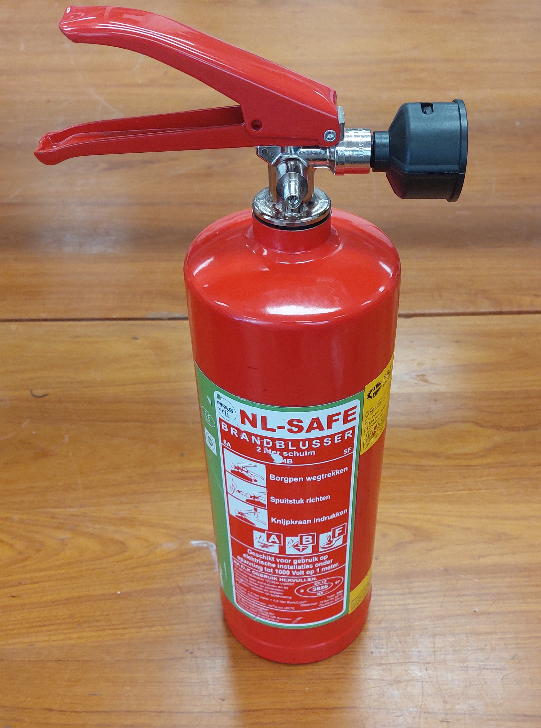
Figure 1:A fire extinguisher is pressured with air, when the air is released the temperature and pressure drops. Once the valve is closed again the pressure and temperature rises. This process allows to calculate the specific heat ratio.
The first part of the process can be described by the Poisson equations for an adiabatic process:
where is the specific heat ratio given by . We note that and . The second part of the process can be described using Gay-Lussac’s relation:
where we consider (again) that and . Rearranging these equations (see Appendix) yields:
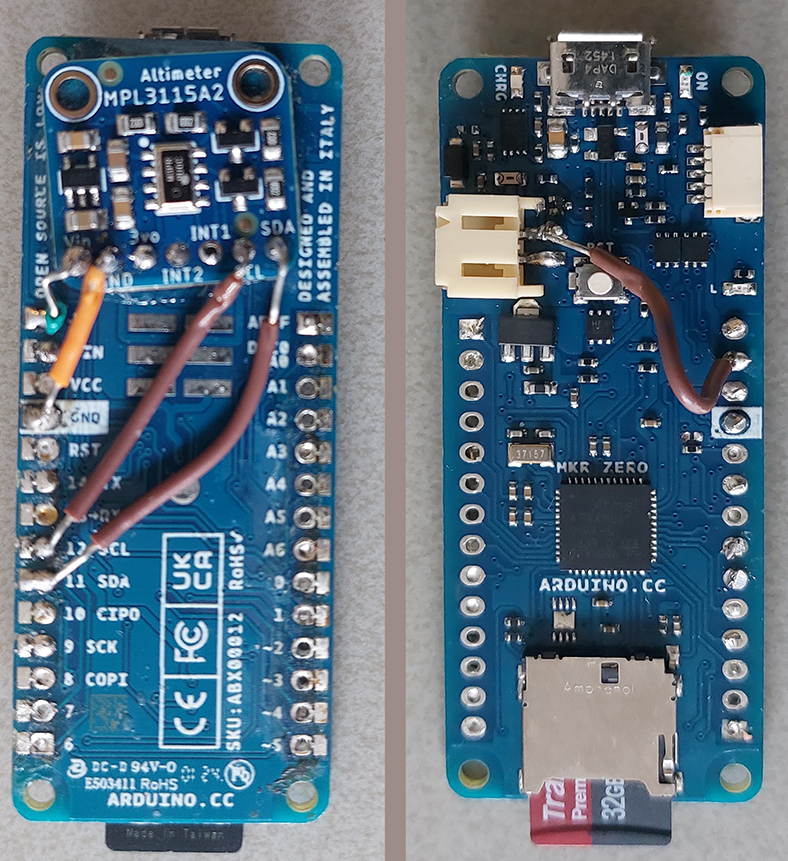
Figure 2:Arduino as logger
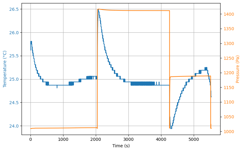
We use an ‘old’ fire fire extinguisher as vessel and a an Arduino MKR Zero with onboard sd-card module as data logger, see {numref}‘fig_experimental_setup_1’. An Adafruit MPL3115A2 is used to measure both temperature and pressure. The sensor is able to detect small pressure changes (+/- 0.05kPa) but is limited in range. The sensor and a LiPo battery are mounted to the Arduino. The entire instrument was then mounted on a regular pvc-tube which is in return mounted on the valve. The results of measuring simultaneously the pressure and temperature when filling the vessel, releasing the air and subsequently closing the valve and waiting for half an hour is shown in Figure 3.
The graph shows the entire thermodynamic process, including the filling of the cylinder at . We note here that due to compression of the gas the temperature increases. Given the educational context, this is a surplus for students to see.
At the valve is opened and the pressure drops in from to . The expected temperature decrease is observed as well (). Once the valve is closed again, we see the pressure in the vessel increases quickly to a maximum of .

Figure 3:some caption
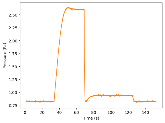
We repeated the measurements with the MPX5700AP absolute pressure sensor which allows to measure at higher pressures, shown in Figure 4. The sensor does not allows for measuring the temperature (which is not needed), but an additional temperature sensor (like the LM35) could be mounted on the Arduino. Using equation (3) we calculated the specific heat ratio. ...

Figure 4:some caption
We should study the pressure temperature relation during pressurization and venting.
We should automate the detection of p1, p2, p3
### Results on measuring the pressure

import numpy as np
import matplotlib.pyplot as plt

data_long = np.loadtxt('brandblusser/TEMP002.csv', delimiter=',', skiprows=1) # lange meting
data_short = np.loadtxt('brandblusser/PRESS001.csv', delimiter=',', skiprows=8) # meerdere metingen op 8 sept, eerste met nozzle, daarna zonder


t = data_long[:,0]*1e-3
temp = data_long[:,1]
pressure = data_long[:,2]

fig, ax1 = plt.subplots(figsize=(8, 5))
#plt.title('Temperature and Pressure vs Time')

color_temp = 'tab:blue'
ax1.set_xlabel('Time (s)')
ax1.set_ylabel('Temperature (°C)', color=color_temp)
ax1.plot(t, temp, color=color_temp, label='Temperature (°C)')
ax1.tick_params(axis='y', labelcolor=color_temp)
ax1.grid()

ax2 = ax1.twinx()
color_pressure = 'tab:orange'
ax2.set_ylabel('Pressure (Pa)', color=color_pressure)
ax2.plot(t, pressure, color=color_pressure, label='Pressure (hPa)')
ax2.tick_params(axis='y', labelcolor=color_pressure)

fig.tight_layout()

plt.savefig('brandblusser/Figuren/temperature_pressure_plot.svg')
plt.savefig('brandblusser/Figuren/temperature_pressure_plot.png',dpi=450)
plt.show()


t_2 = data_short[:,0]*1e-3
pressure_2 = data_short[:,3]

plt.figure()
plt.xlabel('Time (s)')
plt.ylabel('Pressure (Pa)')
plt.plot(t_2, pressure_2, color=color_pressure, label='Pressure (hPa)')


fig.tight_layout()

plt.savefig('brandblusser/Figuren/temperature_pressure_plot2.svg')
plt.savefig('brandblusser/Figuren/temperature_pressure_plot2.png',dpi=450)
plt.show()

# P_1 = max(pressure)
# print(P_1)
# P_b = min(pressure)
# print(P_b)
# P_2 = np.mean(pressure[np.where((t > 5000) & (t < 5100))])
# print(P_2)

# def calculate_gamma(P_1, P_b, P_2):
#     gamma = (np.log(P_1) - np.log(P_b))/(np.log(P_1) - np.log(P_2))
#     return gamma

# gamma = calculate_gamma(P_1, P_b, P_2)
# print(gamma)

# g_1 = (calculate_gamma(P_1+5, P_b, P_2) - calculate_gamma(P_1-5, P_b, P_2))/2
# g_2 = (calculate_gamma(P_1, P_b+5, P_2) - calculate_gamma(P_1, P_b-5, P_2))/2
# g_3 = (calculate_gamma(P_1, P_b, P_2+5) - calculate_gamma(P_1, P_b, P_2-5))/2

# error_gamma = np.sqrt(g_1**2 + g_2**2 + g_3**2)
# print(error_gamma)
Measurements on a syringe
Calibrating our equipment
### BEGIN_SOLUTIONS
# 1. We weten alleen de druk wanneer de volume halveert, dan moet de onbekende volume zo klein mogelijk zijn.
# 2. De druk is dan de atmosferische druk, via het weerbericht te verkrijgen
# 3. Respectievelijk 2*atm en 4*atm.
# 4. Zie hieronder.
# meting op 18 sept, met arduino mkr
import numpy as np
import matplotlib.pyplot as plt
from scipy.optimize import curve_fit
V = np.array([40, 20, 10]) + 1 #mL incl compensatie voor tube
p_ijk = [1017, 2034, 4068] # in mbar
U_ijk = [0.829, 1.452, 2.477] # in V
def linear_fit(x, a, b):
return a * x + b
params, covariance = curve_fit(linear_fit, U_ijk, p_ijk)
U_test = np.linspace(0.8*min(U_ijk), 1.2*max(U_ijk), 100)
pressure = linear_fit(U_test, *params)
plt.figure()
plt.plot(U_ijk, p_ijk, 'ko', label='Ijkpunten')
plt.plot(U_test, pressure, 'r--', label='Lineaire fit')
plt.xlabel('Spanning (V)')
plt.ylabel('Druk (mbar)')
plt.show()
# Tweede meetserie
# volume = np.array([60, 50, 40, 30, 25, 20, 15, 10]) #mL incl compensatie voor tube
# U = np.array([, , ]) # in V
# pressure = linear_fit(U, *params) # in mbar
# def pVrelatie(V, a, dV):
# return a / (V + dV)
# params2, covariance2 = curve_fit(pVrelatie, volume, pressure, p0=[2000, 0])
# v_test = np.linspace(0.8*min(volume), 1.1*max(volume), 100)
# p_test = pVrelatie(v_test, *params2)
# plt.figure()
# plt.plot(volume, pressure, 'o-')
# plt.plot(v_test, p_test, 'r--', label='Fit')
# plt.xlabel('Volume (mL)')
# plt.ylabel('Druk (hPa)')
# plt.show()
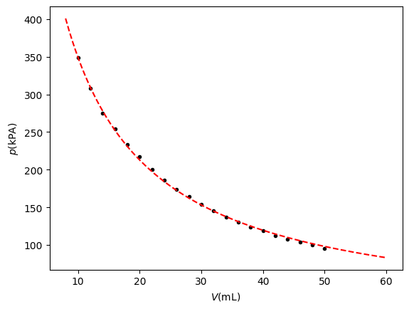
### END_SOLUTIONSHere we reproduce an experiment described in Pols (2024). The setup is shown in spuit, a syringe is connected to the XMP5700AP pressure sensor through a long silicone tube. Starting at 50 mL the pressure is measured at various volumes resulting in the graph of Figure 5.
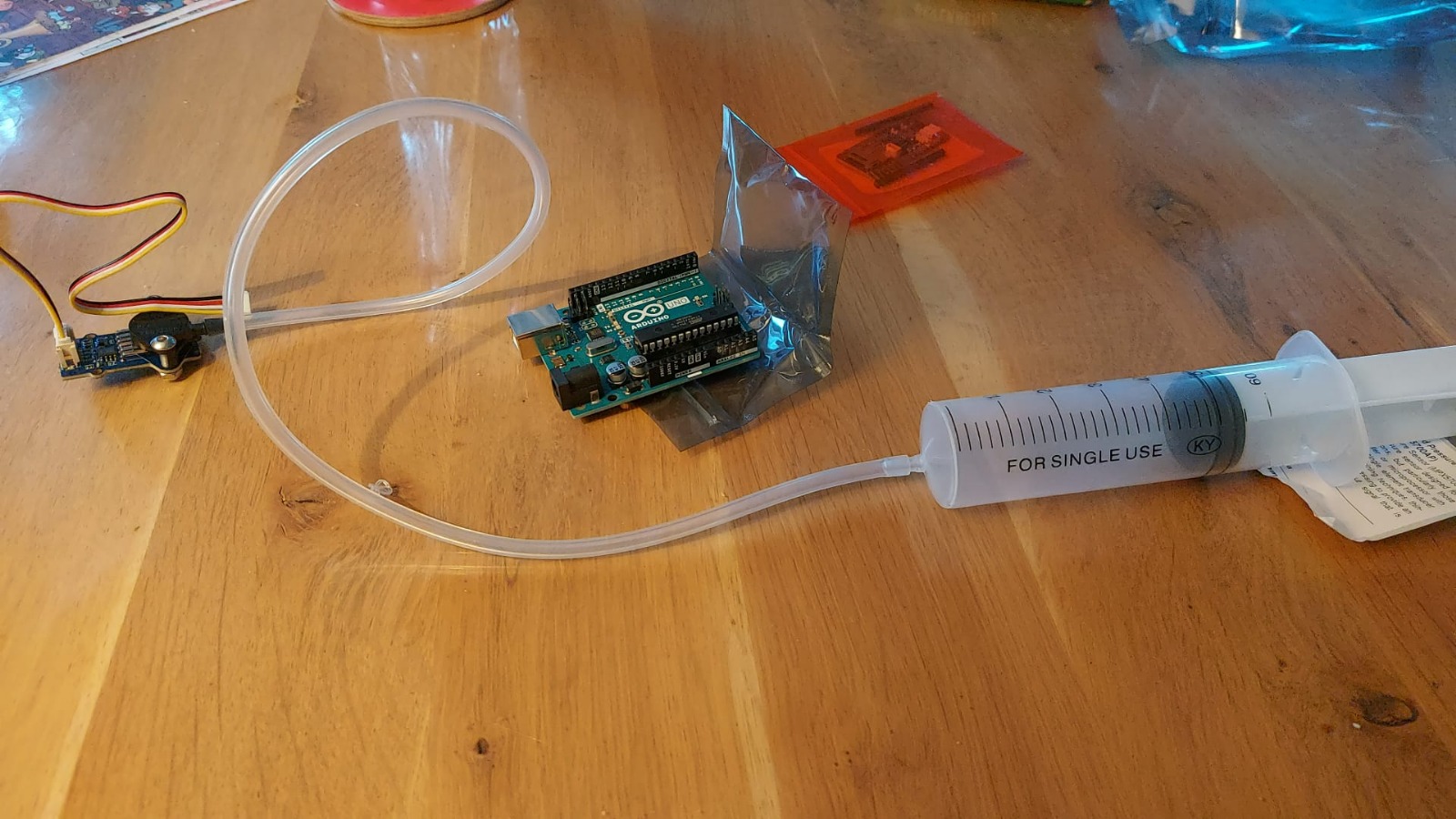
Figure 5:some caption

Figure 6:some caption
import numpy as np
import matplotlib.pyplot as plt
from scipy.optimize import curve_fit

data = np.loadtxt('spuit/metingen.csv', delimiter=';', skiprows=1)

def p(V,a,dV):
    return a/(V+dV)


popt, pcov = curve_fit(p,data[:,0],data[:,1])
print(popt)
V_test = np.linspace(0.8*np.min(data[:,0]),1.2*np.max(data[:,0]),200)
p_test = p(V_test,*popt)

plt.figure()
plt.xlabel('$V$(mL)')
plt.ylabel('$p$(kPA)')

plt.plot(data[:,0],data[:,1],'k.')
plt.plot(V_test,p_test,'r--')
plt.savefig('Figuren/spuitgraph.svg')
plt.savefig('Figuren/spuitgraph.png', dpi=300)
plt.show()
[5450.57035741 5.59439083]
Can it be evaporation?
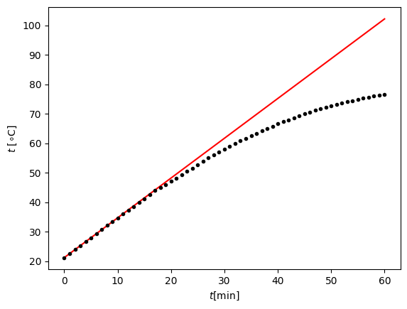
In this task, students were given a dataset of heating water for 60 minutes, as this seemed to be dull and not very educative. The question was whether the difference in expected and measured temperature could be attributed to evaporation. The following are the steps and consideration that should be taken by the students.
Figure X shows the measurements and the expected temperature rise of the water if not accounted for losses and evaporation. It clearly shows a deviation from the measured temperature above 50∘C, reaching a total temperature difference of 25.6∘C. The difference between the mass of water before and after the experiment was 18±1 gram, corresponding to a total heat of evaporation of 40.6 kJ (of the total supplied energy 160 kJ). A first estimate () would result in a temperature of 6.2 K. Based on these findings, students were asked to devise a better experiment to come to understand the thermodynamic process that is taken place (e.g. a continuous measurement of the total mass and temperature).
Next, students were asked to use the data to build a numerical simulation where they could simulate both the temperature rise and the evaporation of water.
Source
import numpy as np
import matplotlib.pyplot as plt

# Inladen en plotten van de data
data = np.loadtxt("verdamping/tempmetingen.csv", delimiter=";", skiprows=1)

time = data[:,0]
temperature = data[:,1]


m_w_b = (1292.9 - 820.8)*1e-3
m_w_e = (1274.9 - 820.8)*1e-3
d_m_w = m_w_b - m_w_e
print(d_m_w)

c_w = 4186 #J/(kg K)

# Berekenen van totale toegevoerde energie op basis van opwarming in eerste 10 minuten waarbij we verwachten dat er nog nauwelijks warmte in verdamping gaat zitten
Q_totaal = c_w*m_w_b*(temperature[10]-temperature[0])/10*60
print(int(Q_totaal),"J")

# Berekenen van verwachte eindtemperature, zonder verdamping of warmteverlies
dt_verwacht = Q_totaal /(c_w*m_w_b)
t_verwacht = dt_verwacht + temperature[0]
dT = round(t_verwacht-temperature[-1],1)

print(t_verwacht)
print("verschil in temp: ", dT , "K")

plt.figure()
plt.xlabel("$t$[min]")
plt.ylabel(r"$t$ [$\circ$C]")

plt.plot((time[0],time[-1]),(temperature[0],t_verwacht),'r-')
plt.plot(time,temperature,'k.')
plt.show()


# verdampingswarmte bij standaardomstandigheden (temperature verandert, dus dit is geen goede aanname)
H_w = 2256e3 #J/kg

# verwachte eind temperature als we verdamping eraf halen
Q_verd = d_m_w * H_w
print(Q_verd)
t_e = (Q_totaal -Q_verd)/(c_w*(m_w_b+m_w_e)/2)+temperature[0]
print("Het verschil is nu nog maar:", round(t_e-temperature[-1],1), "K")
0.01799999999999996
160073 J
102.20000000000003
verschil in temp:  25.6 K
40607.99999999991
Het verschil is nu nog maar: 6.2 K
Discussion & Conclusion
Our aim was to devise a cheap (scalable) but accurate experiment in the topic of thermodynamics. Determining the specific heat ratio using the valve of a fire entinguisher and an arduino as logger ... more process than expected (filling)
Appendix
Setup and assumptions
Ideal gas in a rigid vessel of volume .
State (1): initial equilibrium at .
Rapid vent to atmosphere (no heat exchange during the short release) to State (2): pressure equals barometric pressure , temperature drops to .
Valve is then closed; gas reheats at constant volume (no work) back to , reaching State (3): pressure .
The quick release (1)(2) is adiabatic; the recovery (2)(3) is isochoric.
Step 1 — Adiabatic release (1)(2)
For a reversible adiabatic process of an ideal gas,
Thus,
Step 2 — Isochoric reheat (2)(3)
At constant , . Hence,
Step 3 — Eliminate and solve for 
Insert (A2) into (A1) and cancel :
Take natural logs and rearrange:
This matches the expression quoted in the main text, with .
- Millar, R., Le Maréchal, J.-F., & Tiberghien, A. (1999). “Mapping” the domain - varieties of practical work. In J. Leach & A. C. Paulsen (Eds.), Practical work in science education (pp. 33–59). University of Roskilde Press.
- Pols, C. F. J., & Dekkers, P. J. J. M. (2024). Redesigning a first year physics lab course on the basis of the procedural and conceptual knowledge in science model. Physical Review Physics Education Research, 20(1). 10.1103/physrevphyseducres.20.010117
- Hut, R. W., Pols, C. F. J., & Verschuur, D. J. (2020). Teaching a hands-on course during corona lockdown: from problems to opportunities. Physics Education, 55(6), 065022. 10.1088/1361-6552/abb06a
- Pendrill, A.-M., & Eager, D. (2020). Velocity, acceleration, jerk, snap and vibration: forces in our bodies during a roller coaster ride. Physics Education, 55(6), 065012. 10.1088/1361-6552/aba732
- Pols, F. (2024). Show the Physics. TU Delft OPEN Publishing. 10.59490/tb.101