01 Mathematical Pendulum (1) Simple Harmonic Motion

Aim¶

To show the relationship between position, velocity and acceleration of a simple pendulum.

Subjects¶

• 3A10 (Pendula)

• 3A40 (Simple Harmonic Motions)

Diagram¶

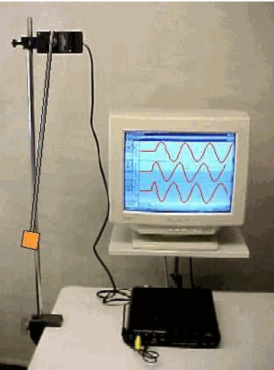
Equipment¶

• Simple pendulum: aluminum tube with brass mass.

• Rotary motion sensor (we use Pasco CI-6538).

• Data-acquisition system and computer with software (we use ‘Science Workshop’).

• Projector to project the monitorscreen.

Presentation¶

Set up the software to display graphically angular position, angular velocity and angular acceleration of the pendulum. When the pendulum is in its vertical position at rest, we start data collection. We give the pendulum a small amplitude and let it swing. When we have collected about four complete cycles, the data-acquisition is stopped.

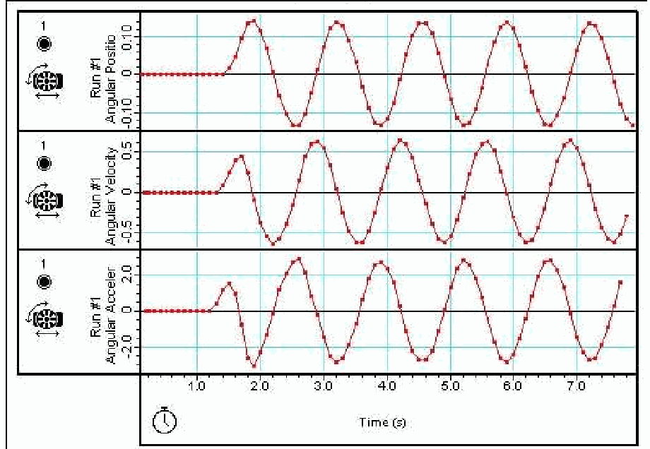
Already at first glance this registered graph shows its sine-shaped appearance. To have a more convincing conclusion the software can apply a mathematical curve-fit to the registered position-graph, to show that a sinusoidal equation “covers” the position-graph very good. So a sine-function describes the behavior (position-time) of this pendulum very good. A second run of the oscillations is registered, but now with a higher amplitude. Clearly can be observed now that the motion is no longer sinusoidal Trying a sine-fit will confirm this (read the chi2-value). Make a third run again with small amplitude and check the differential relationships between ‘position’, ‘velocity’ and ‘acceleration’: e.g.

• The points of zero-velocity correspond with maximum - and minimum position;

• The acceleration-graph is an inverse “copy” of the position-graph;

• ……….

Explanation¶

The equation that describes the motion of the mass $m$ is given by $a_{x}=\frac{d^{2 s}}{d t^{2}}=-g \sin \theta$.

This is not a simple harmonic motion since $\sin \theta$ is not proportional to $s$.

Only for small amplitude oscillations $\sin \theta \approx \theta=\frac{s}{l}$ and the equation of motion reduces to $\frac{d^{2} s}{d t^{2}}=-\frac{g}{l} s$ This is the differential equation for simple harmonic motion, giving our observed sinusoidal graphs.

For further explanation see: SourcesXX.

Sources¶

• Mansfield, M and O’Sullivan, C., Understanding physics, pag. 48-52

• Young, H.D. and Freeman, R.A., University Physics, pag. 398-399