04 Chaotic Pendulum - The Demonstration Laboratory

Aim¶

To analyze the chaotic motion of a parametrically driven pendulum by explaining its motion in phase space by making a Poincaré plot.

Subjects¶

3A10 (Pendula)
3A95 (Non-Linear Systems)

Diagram¶

Equipment¶

Parametrically driven pendulum
Photogate
Rotary motion sensor
Data-acquisition system and computer. (We use Science Workshop).
Projector to project monitor-image.

Presentation¶

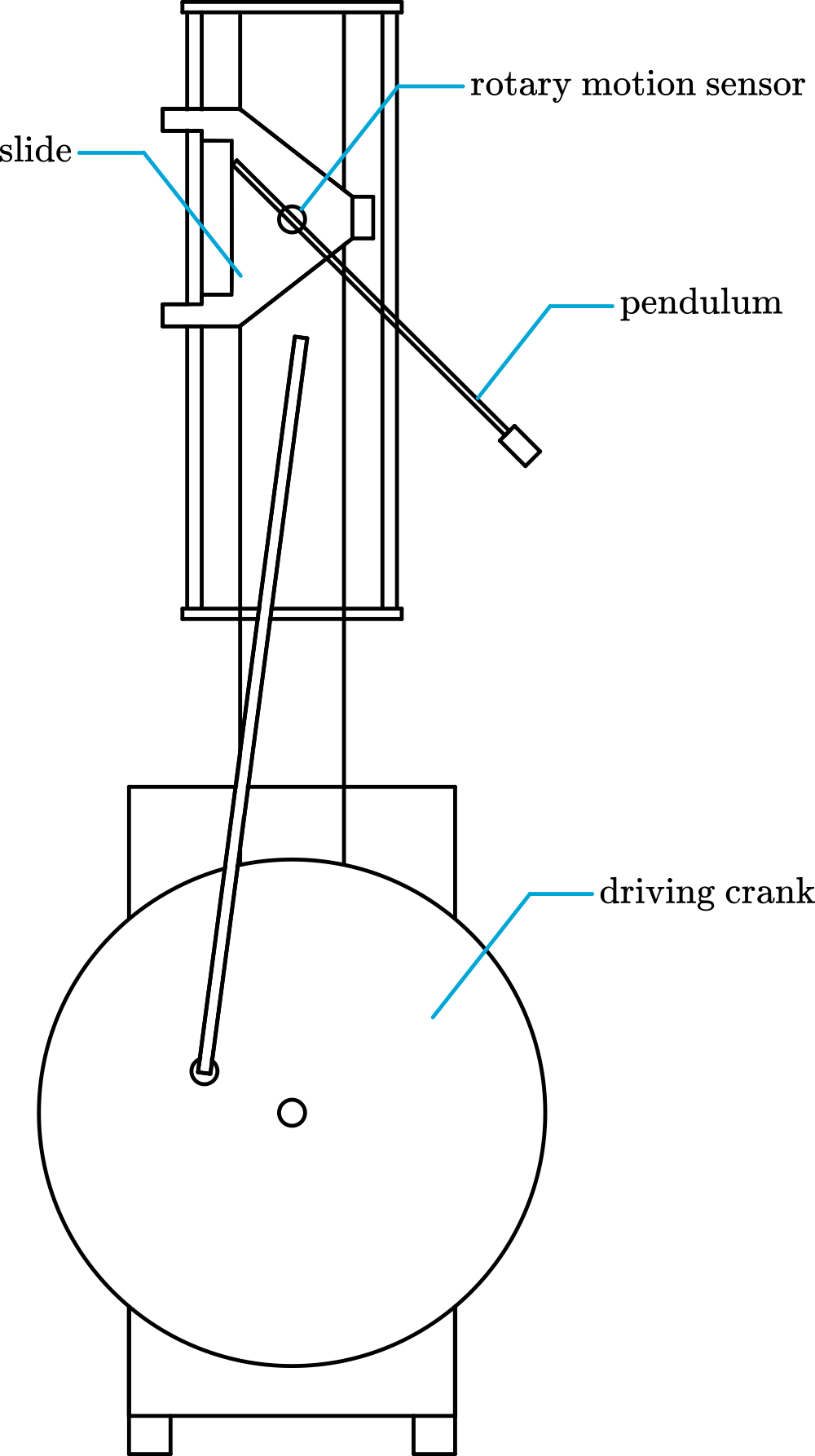
The Pendulum is fixed on the shaft of the rotary motion sensor. The rotary motion sensor is fixed to the slide that is driven up and down by a crank mechanism (See Diagram and Figure 3 1).

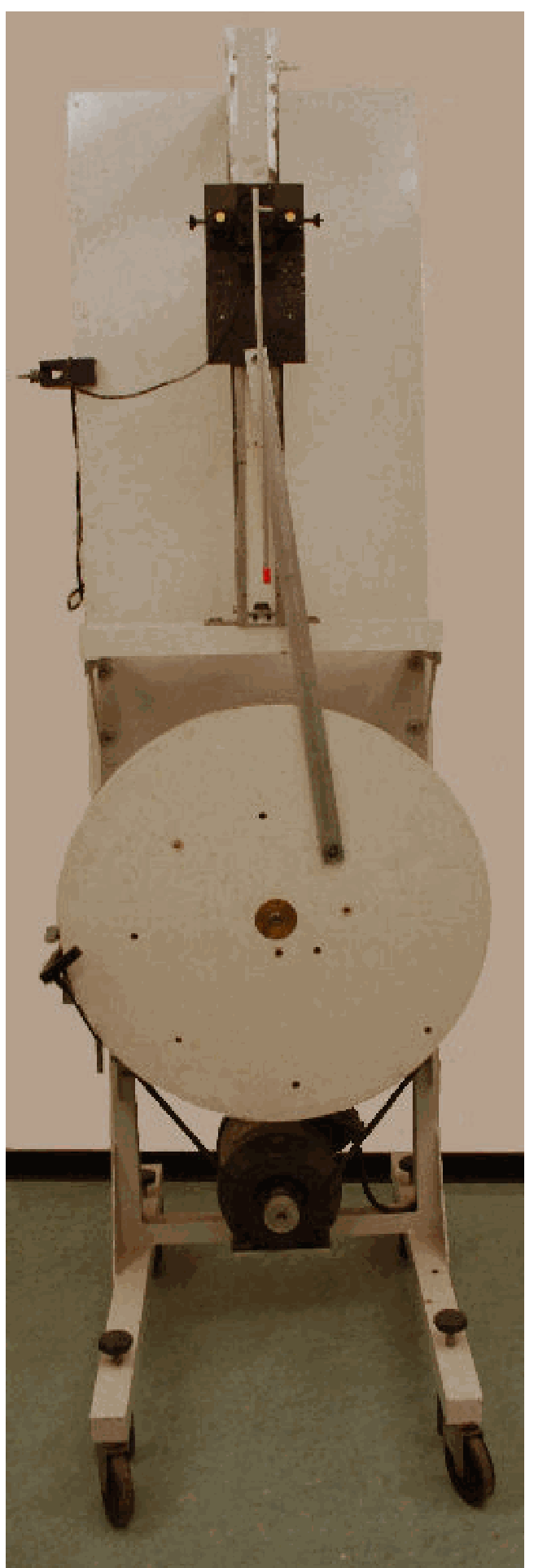
The driven pendulum, see Figure 2, is placed on a spot that can be observed by all the students but which can be closed off during the lecture i self. Place it for example just outside the lecture room, so the door can be shut during the lecture, while keeping the monitor image visible to the students

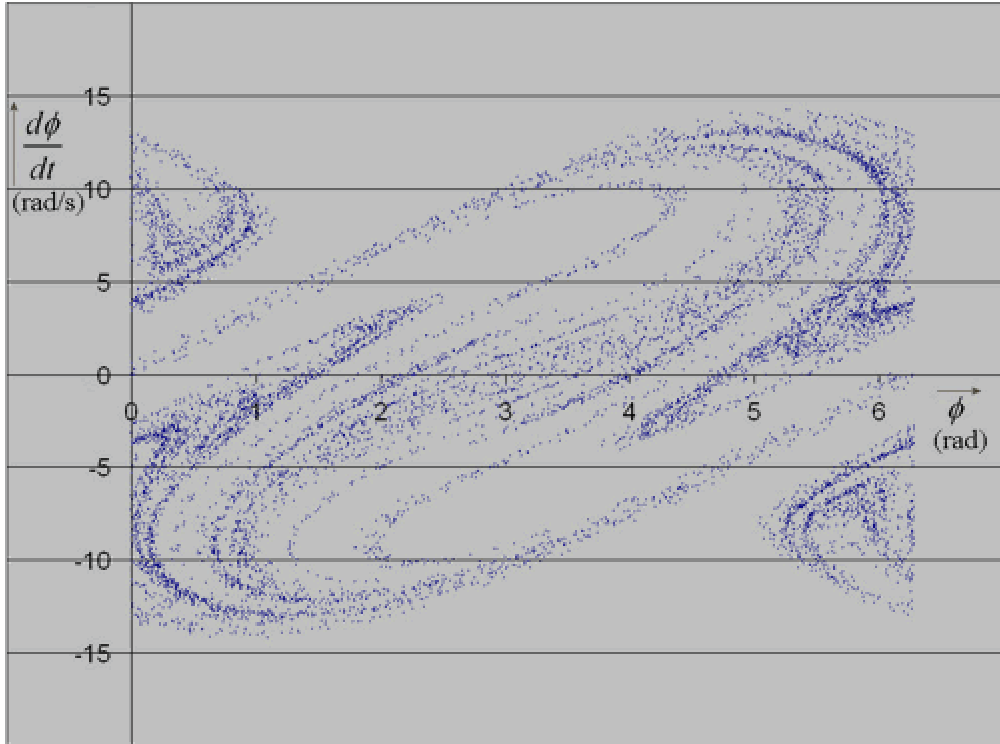
The software is set up to make a Poincaré plot of the angular position and angular velocity, and will be projected in the lecture room with use of the projector. The Poincaré plot will grow during the lecture and after a while the strange chaotic attractor will be displayed. In about 1 hour you will be able to see the contours of the attractor; after an other hour you will have a plot like in Figure 3.

At the beginning of the lecture, having started the driven pendulum, you can introduce the driven pendulum and show its chaotic behavior. After this you can explain why we use a Poincaré plot to analyze the chaotic movement of the pendulum and that in a Poincaré plot not the time but space determines when to plot a point, by showing the students the spot where both angular position and angular frequency is measured en plotted against each other in the Poincaré plot.

Explanation¶

The equation of motion of a Chaotic pendulum is (see: SourcesXX):

\frac{d^{2} \vartheta}{d t^{2}}+\frac{k_{2}}{m L^{2}} \frac{d \vartheta}{d t}+\left[\omega^{2}-\frac{A \Omega^{2}}{L} \cos (\Omega t)\right] \sin (\vartheta)=0

(1)

where:

$k_{2}$ : damping constant
$m$ : mass of the pendulum
$L=\frac{I}{m \ell}=\frac{\left(k^{2}+\ell^{2}\right)}{\ell}$ : reduced length of the pendulum
where $I$ is the moment of inertia of the pendulum with regard to its suspension point, $\ell$ is the distance between the point of suspension and the centre of mass, (see: McComb §6.2.8), and $k=\frac{\int r^{2} d V}{\int d V}=$ (the radius of gyration of the pendulum, see: McComb §6.2.2)
$\omega=\sqrt{\frac{g}{L}}$ (eigen frequency of pendulum at small amplitudes)
$A$ : amplitude of the nearly harmonic driving force
$\Omega$ : angular driving frequency.

If there is no damping, $k_{2}=0$ . If there is no driving force, $A=0$ . Then the equation of motion will be:

\frac{d^{2} \vartheta}{d t^{2}}+\omega^{2} \sin (\vartheta)=0

(2)

When we substitute, $\omega=\sqrt{\frac{g}{L}}$ and $L=\frac{I}{m \ell}$ , we will get the following equation of motion:

\frac{d^{2} \vartheta}{d t^{2}}+\frac{m g \ell}{I} \sin (\vartheta)=0

(3)

Solving this differential equation yields:

\frac{1}{2} \vartheta^{2}-\frac{m g \ell}{I} \cos (\vartheta)=\text { const. (McComb equation 6.25). }

(4)

The Parametrically driven pendulum is based on the article, *Unstable periodic orbits in the parametrically excited pendulum, of W. van der Water.*In this article some more friction terms have been added to the equation of motion of the chaotic pendulum, so that result of the simulation and the actual experiment are more like each other.

Remarks¶

The pendulum is mounted on the Rotary motion sensor which is mounted on the slide and while provide use with the both the angular position and angular velocity (see Figure 4).

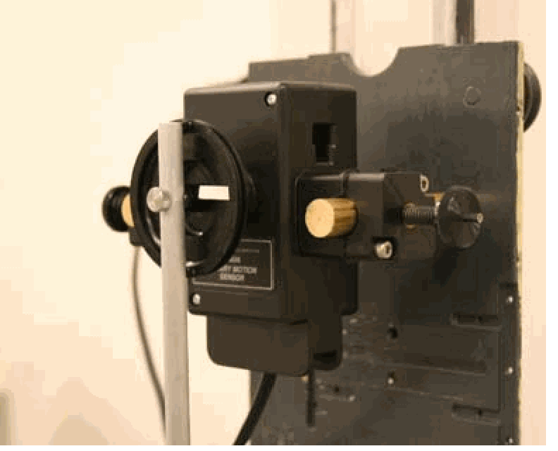
The Photogate is placed on driving wheel and will give use the moment at which we will plot both the angular position and angular velocity of that moment in the Poincaré plot (see Figure 5).

Test if the driven pendulum keeps his chaotic movement for the period you want to use it, it sometimes ends in a harmonic movement after a while. When this happens try to adjust the driving frequency of the pendulum
As extra you could ask the students to make a simulation of this pendulum using Maple or Mathlab.
Then you need to know the following parameters of the pendulum:
angular driving frequency $\approx 9 \mathrm{rad} / \mathrm{s}$
amplitude of the driving force $\approx 0.125 \mathrm{~m}$
length of the pendulum $\approx 0.3 \mathrm{~m}$
mass of the pendulum $\approx 0.03 \mathrm{~kg}$
damping constant $\approx 1.7 \times 10^{-5} \mathrm{~S}$

Sources¶

Dynamics and Relativity, W.D. McComb, pag 125-128
Unstable periodic orbits in the parametrically excited pendulum, W. van de Water; M. Hoppenbrouwers; F. Christiansen, Phys. Rev A 44(1991)6388698
The Pendulum, A case study in physics, G.L.Baker J.A.Blackburn, pag. 121-149

3A10 Pendula

03 Mathematical Pendulum (3) Determining g

3A15 Physical Pendula

01 Physical Pendulum (1) Compound Pendulum