Aim
To verify Kepler’s second law
Subjects
1L20 (Orbits)
8A10 (Solar System Mechanics)
Diagram
Equipment
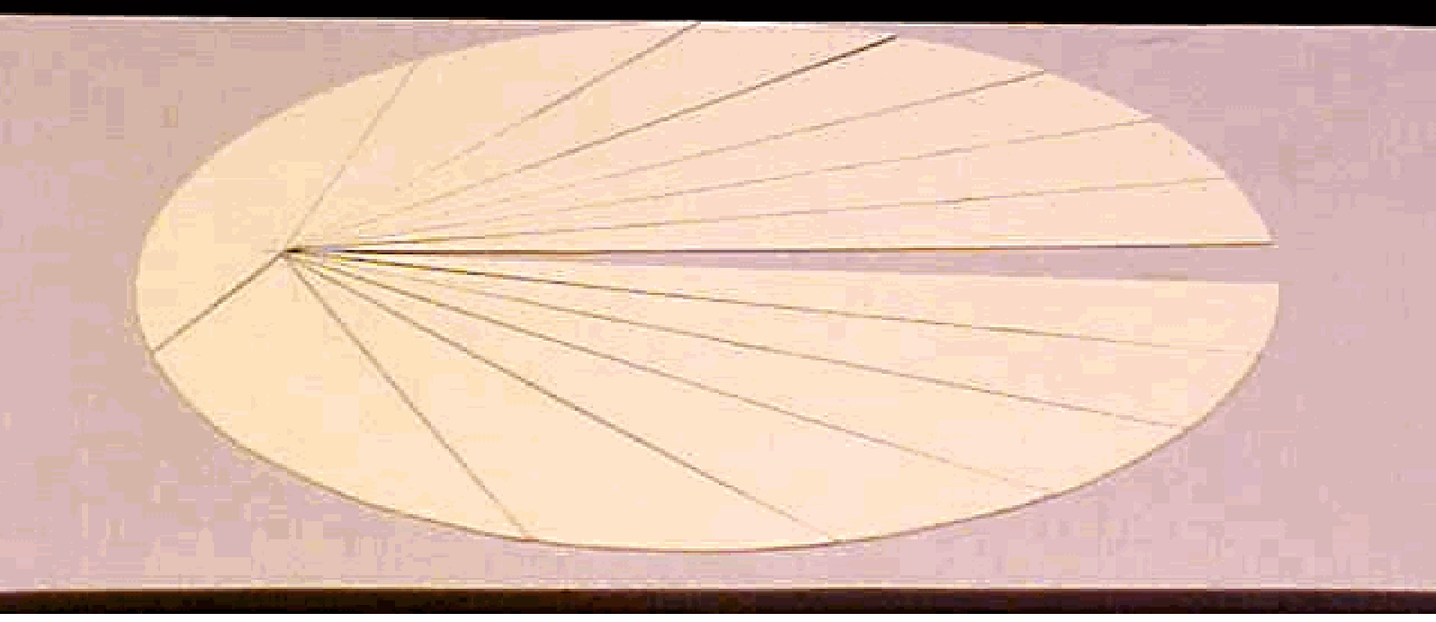
Board-model with “Kepler-areas” (see Diagram).
Balance, with large display.
Software program (we use Interactive Physics) drawing the position of a planet around a central mass at a couple of time-intervals.
Projector, to project the monitor-image on a large screen.
Presentation
By means of the software program an elliptical orbit is projected (see Figure 2A). The speed in the orbit is visualized when in the orbit points are plotted at constant time-intervals. This orbit is also plotted when the time-interval applied is 16 times larger (Figure 2B).
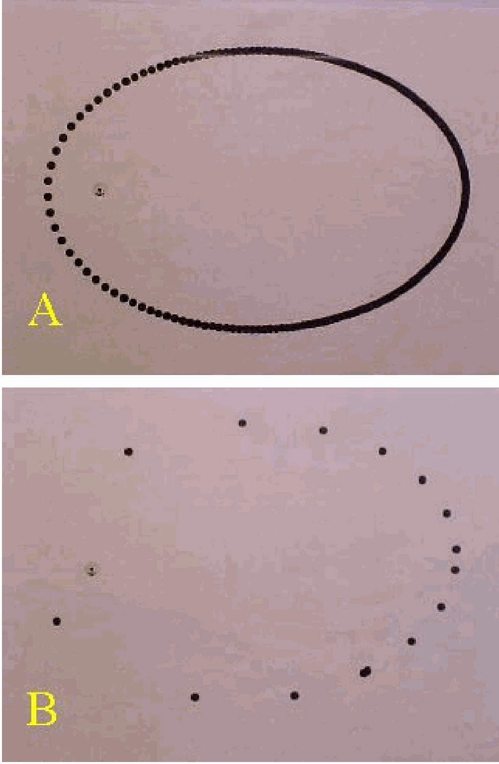
Before, we had this figure projected on a large sheet of cardboard and the elliptical time-segments were cut out (see Diagram). The similarity between the software-image and the cardboard-model is shown to the students. When the segments are placed one after the other on the balance, equal mass is observed. This also means that the areas of the segments are equal (Kepler’s second law).
Explanation
Kepler “found” his law while working on the astronomical data of Tycho Brahe. So in our demonstration the law should arise from watching the areas and “seeing” the equality. Since Newton we can use the law of conservation of angular momentum. Using this law we can explain the statement of Kepler’s second law.
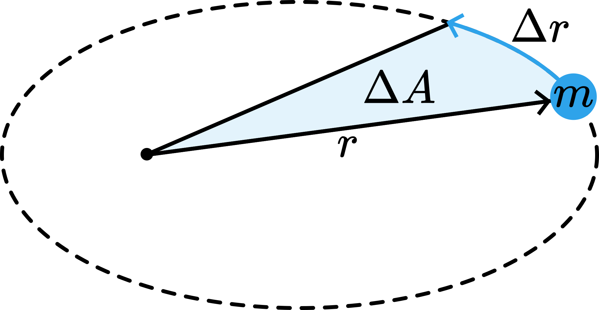
Consider the area in Figure 3 swept by the vector in a time .
Since
So, when is constant (equal time-intervals), then is constant.
Simulations
On the internet you can find many simulations that are appropriate. For instance on:
Remarks
being constant means also that moves in a fixed, flat plane, since will not change its direction
Sources
Mansfield, M and O’Sullivan, C., Understanding physics, edition 1998, pag. 105-106.
McComb,W.D., Dynamics and Relativity, edition 1999, pag. 71.
Roest, R., Inleiding Mechanica, vijfde druk, pag. 100-102.
Stewart, J, Calculus, edition 1999, pag. 866-867.