Goal
In this experiment, we will study the light emitted by a mercury lamp (Hg) and sodium (Na). The spectrum for such lamps is comprised of a few clear spectral lines. The goal for this experiment will be to determine the wavelengths of those lines as accurately as possible. We will use a diffraction grating to do so. One of the questions related to this experiment is: how small can the difference in wavelength of two spectral lines be for those lines to still show up separately on the setup?
Preparation
Before you arrive at the practical, you are expected to have properly studied this chapter of the manual, and to have written down the answers to the twelve questions that are noted in your lab journal. If any questions came up during your preparation, write them down in your journal and ask them at the beginning of the experiment.
Theoretical Background
What is a diffraction grating?
A diffraction grating is a plate with a very large number of parallel lines on it, which are spaced an equal distance from each other. A schematic representation is shown in Figure 1.
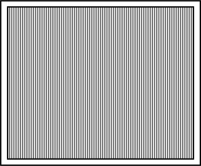
Figure 1:Schematic representation of a diffraction grating. Typical measurements are 5x5 cm. The number of lines per mm is in the range 100-1000.
Typical measurements are 5x5 cm and a typical value for the number of lines per mm is in the range 100-1000. A diffraction grating can be either transmissive or or reflective, known, respectively, as a transmission or a reflection grating.
What does a diffraction grating do?
A diffraction grating is an optical instrument which diffracts light. The larger the wavelength, the larger the diffraction. Figure 2 shows what happens when ‘white’ light with a continuous colour spectrum between blue and red falls on a transmission grating. A part of the light goes straight ahead and remains white. This is the order diffraction pattern. Under and above of this order we see spectacular ribbons of which show a colour range from red to blue". These are the order diffraction patterns. These patters can repeat itself multiple times ( order, order, ...).
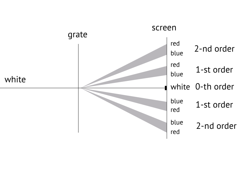
Figure 2:A transmissive grating in operation. White light with a continuous colour spectrum from blue to red is split into multiple colours and orders.
The purpose of a diffraction grating is to study the colour spectrum of a light source. As seen in Figure 2, the vertical distance on the screen is a measurement for the wavelength of a certain colour. A diffraction grating also allows one to select a desired colour from white light.
Light rays and wavefronts
This experiment focuses on the wave characteristics of light. The terms interference and diffraction are central to this. The Huygens Principle is often used to explain diffraction phenomena. This principle relates to the extension of wavefronts. A wavefront is a collection of points where the “vibration” is in the same phase. Waves in water are in fact wavefronts. If we throw a stone into the water, then we see wavefronts that extend in a circular fashion. If we look at waves washing up at the beach, we see a series of parallel wavefronts. These characteristic wavefronts are shown schematically in Figure 3.
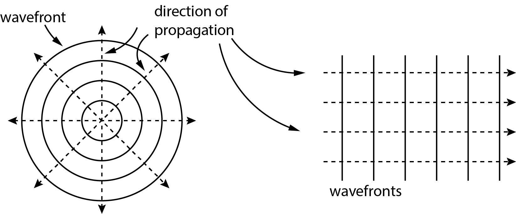
Figure 3:Two characteristic wave patterns. Left: the extension of circular (spherical) shaped wavefronts. Right: plane (flat) waves moving to the right (= parallel light bundle).
The relation with light rays is that the propagation direction of the light in a certain point is displayed by a light ray. If a wave propagates in an isotropic medium, then the direction of it is perpendicular to the wavefront. See Figure 3.
Huygens principle (Wolfson, ch. 32.5)
All points on a wavefront work like point sources for spherically shaped ‘waves’ which propagate with lightspeed in the medium. A short time later, a new wavefront is formed by the surface that touches all ‘waves’ which propagate in the previous direction of propagation.
Figure 4 shows how this works. On the left we see how a spherically shaped wavefront at develops itself to a new spherically shaped wavefront at . For four points on the wavefront at is shown how the waves develop themselves in a time interval . The new wavefront at is the ‘tangent’ line to these waves.
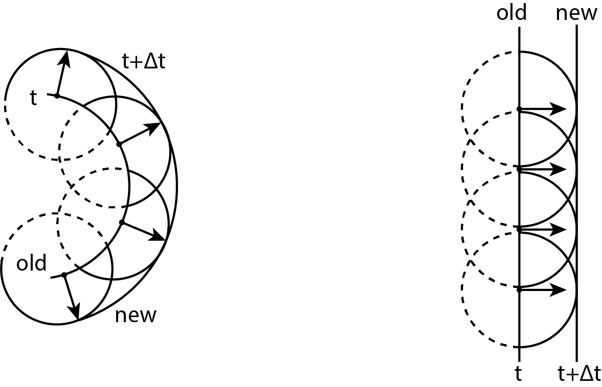
Figure 4:Propagation of a wavefront according to the Huygens principle. Left a spherically shaped wavefront and right a plane wavefront.
The image on the right in Figure 4 displays the same way of propagation for a plane wavefront. As said, the Huygens Principle explains the diffraction of light. For the first application, we look at what happens when a plane wave falls on a screen with a hole in it. The diameter of the hole is comparable with or smaller than the wavelength of the light. See Figure 5.
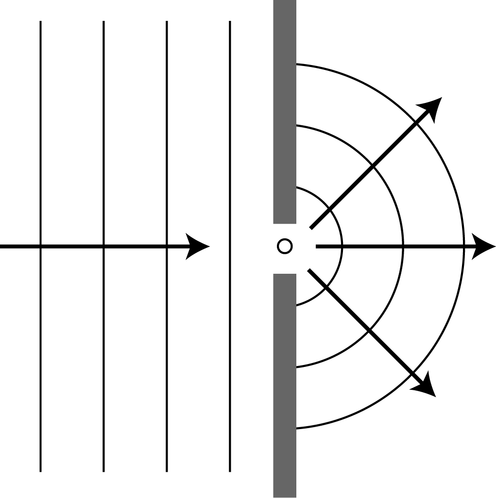
Figure 5:A plane light wave falls on a screen with a hole with a diameter comparable to the wavelength. According to the principle of Huygens, the hole acts like a point source that emits spherically extending waves.
In Figure 5 a plane wave falls on the screen from the left side. The light that falls in the hole, emits spherically propagating waves according to the Huygens principle. If the size of the hole is of the same order as the wavelength, most of the light is diffracted. To see a demonstration with a tank filled with water, look up ‘ripple tank diffraction’ on YouTube. In Fig. 32.33 (c) of Wolfson & others (2007) you can also see how the intensity of the light.
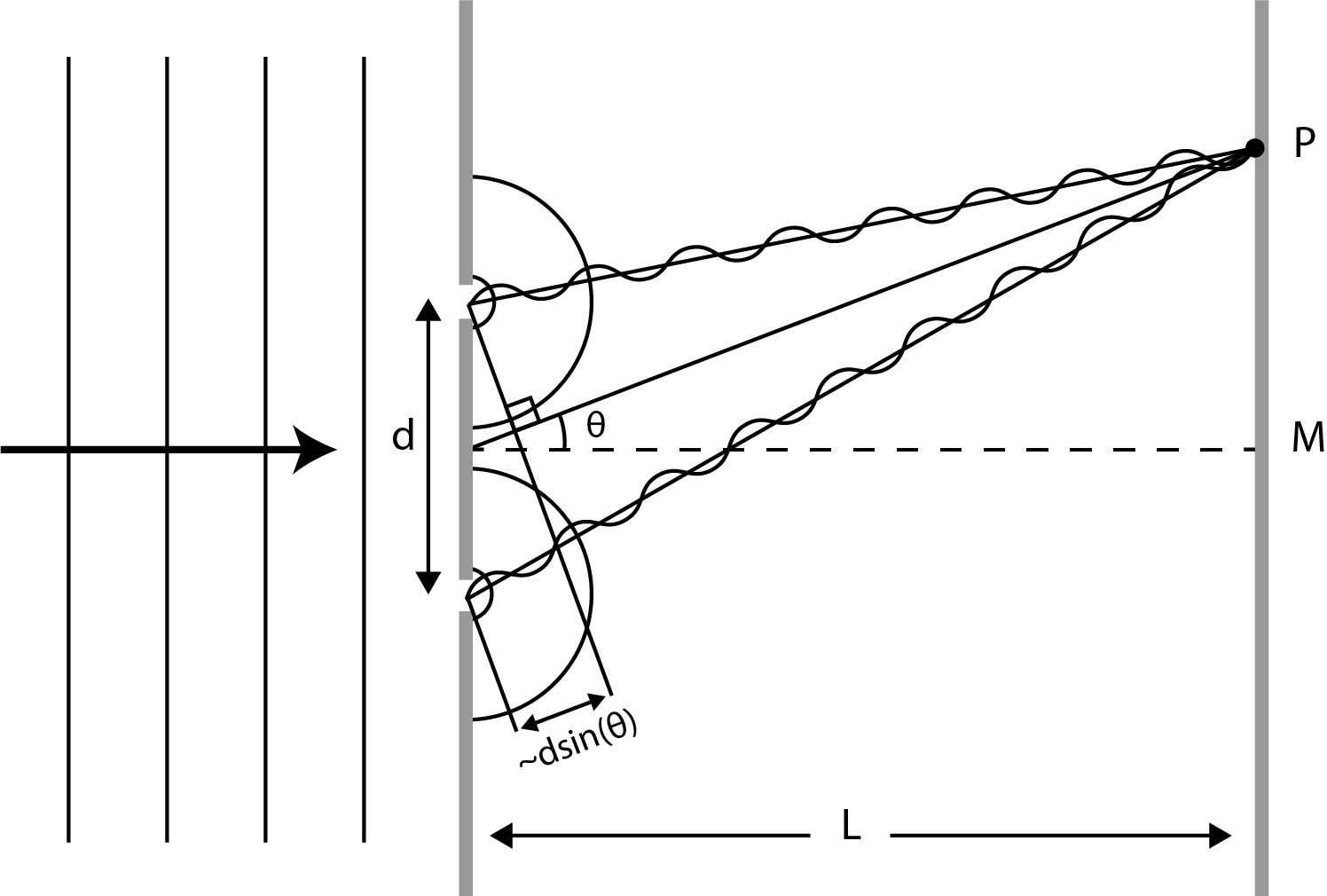
Figure 6:A plane light wave falls on a screen with two holes. These holes work like point sources that emit spherically propagating waves in phase. Both waves interfere constructively in point P in this situation.
Interference
The next question is: what happens if there are two holes in the screen? This is shown in Figure 6 where a plane wave falls perpendicularly from the left side on a screen with two holes (diameter wavelength). The distance between the holes, , is three times the wavelength for instance. The plane wave causes the holes to emit spherically shaped waves in phase. The light in a point P (See Figure 6) is a superposition of the light that is emitted by the two sources. Both sources of light interfere with each other. The distance between the upper hole and P that is covered by the light is not the same as the distance between the bottom hole and P covered by the light. The length of the path covered by the light is different, meaning that the phase of the two waves at P is not equal. However, it is possible that the phase difference is exactly the same as a whole number times , as shown in Figure 6. The phase difference is and the waves interfere constructively in P. For points just above and below P, the phase difference is different and there is no longer 100% constructive interference. Thus the light intensity will be lower.
Light from both sources arrive at point M. What is the path (phase) difference? What does this mean in terms of constructive or destructive interference? Does this depend on the wavelength of the light?
It can be deduced from Figure 6 that the path difference can be approached by . The angle determines the place of P (and vice versa). Constructive interference occurs when:
with an integer that we call the order.
can also be negative. What does this mean for ? What is the location of P in this case?
What consequences does a change in and/or have on the angle in the case of constructive interference?
Interference in “a point far away”. Multiple sources.
In Figure 6 the distance between the screen and a source is of the same order as the distance between two sources. This concerns distances of the order 10 . In practice we work with distance in the range of . So, we are interested in what happens in points that are far away from the sources.
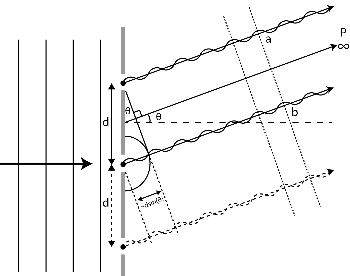
Figure 7:The upper part of this figure is identical to Figure 6, the only difference is that the point P is now infinitely far away from the sources. There is constructive interference in point P. The bottom right part of the figure shows that extra holes with spacing also contribute to the constructive interference. The slanted striped lines on the right side of the figure indicate the development of plane wavefronts (parallel bundle).
Figure 7 shows that the paths from the sources towards P now run parallel to each other. Because of this, the condition for constructive interference (eq. (1)) is exact.
It is not hard to imagine what happens if we add an extra hole. We make sure the third hole is located on the line that goes through the two other holes and that the mutual distance is (see Figure 7 above). The third source also emits, in phase, a wave that contributes to the amplitude in the far point P. The correlated path runs parallel to the other path. The path difference is or . So the contribution of the third source interferes constructively with the other sources.
We can continue this reasoning for holes that lie on a line with mutual distance d. In this manner we construct the theoretical description for a diffraction grating with lines. The amplitude of the electric (magnetic) field of the light in P is times as large as the amplitude that is produced by a single hole.
If we look at Figure 7, it is tempting to drawn lines that go through the points where the drawn waves run in phase (the dotted lines on the right side in Figure 7). These lines are perpendicular to the direction of propagation and you might be inclined to conceive these lines as wavefronts of a parallel bundle. That thought is fine, but you must be sure that for instance the points on the dotted line between the points a and b (in Figure 7) vibrate in phase with the vibrations in a and b. Close to the sources this is a difficult matter, but far away from the sources this is certainly the case. You can determine this using Huygens’ principle. This also follows from the wave equation. For light waves that are possible in a uniform medium, the direction of propagation is always perpendicular to the wavefronts.
From transmission to reflection grating. Grating equation.
Up until now, we have discussed the operation of a diffraction grating according to a transmission grating. However, reflection gratings are more commonly used. These have accurate grooves instead of translucent lines. Everything that has been said above about plane waves, point sources, including (1) is also true for reflection gratings.
At the derivation of eq. (1) it is assumed that the incoming plane wave falls perpendicular into the diffraction grating. That restriction does not have to be made. The plane wave can also fall at an angle with the normal of the diffraction grating. Figure 8 demonstrates how the angles of the exiting bundles can be found for a parallel bundle that falls at angle with the normal of the diffraction grating.
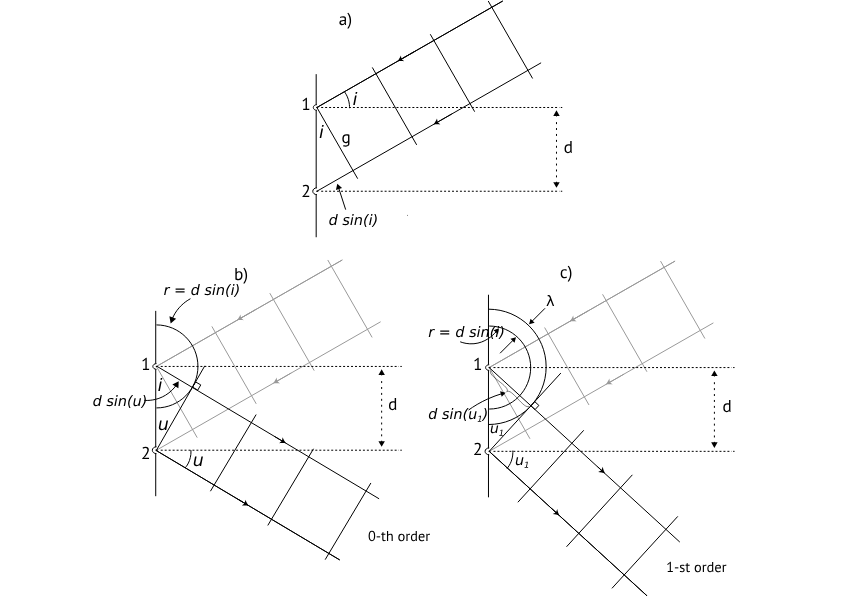
Figure 8:construction of the angle of reflection for a reflection grating. a) a plane wave falls at an angle onto the diffraction grating. The wavefront g reaches grating line 1. This incites the development of a spherical wavefront from 1. A time interval later reaches the plane front g grating line 2. b) at this point the spherical wavefront from 1 has the radius . The vibrations on this wavefront and the ones in point 2 are in phase. The line that goes through 2 and touches the spherical wavefront determines the direction of propagation of the 0-th order exiting wavefronts (wavefront is perpendicular to direction of propagation) and c) the construction of the direction of the 1-st order exiting bundle.
In Figure 8a, a parallel bundle falls at an angle with the normal of the diffraction grating. A plane wavefront will first reach grating point 1 and, according to Huygens, that point emits spherically shaped waves. A time later the wavefront reaches grating 2. From Figure 8a it turns out that ( is the distance between two grating lines and is the speed of light). In Figure 8b we see how far the spherical wave from grating point 1 has propagated. As said, the phase of points on a wavefront is by definition equal, but in this case the vibration in grating point 2 is also in the same phase. We can now draw a line which goes through grating point 2 and touches the spherical wave. This line is cut by the perpendicular line that goes through grating point 1 and the point where the first line touches the spherical wave. These two lines can be seen as the “precursors” a wavefront / direction of propagation pair before the exiting wave (as discussed at Figure 7). Just like in Figure 7 more grating lines can be added to this consideration.
Figure 8b is special because in the way that it turns out from the figure that . In this case the exiting bundle is called the 0 order diffraction bundle.
Of course not only the drawn wavefront in Figure 8b has the same phase as the phase in grating point 2. Wavefronts belonging to spherical waves that have left earlier,have the phase as the phase in grating point 2 as well (apart from a difference of of course). In Figure 8c you can see a bundle emerge from the sketching of the tangent line on the wavefront with radius . It turns out from the figure that in this case . Of course we can also do this for wavefronts with radius , with an integer. For an incident angle we can determine the angles from possibly exiting bundles with:
This is the grating equation. It follows from this equation that, if a plane wave with a certain wavelength falls on the diffraction grating under an angle , different plane waves are reflected with the same wavelength under different angles . We can determine the wavelength of a certain component by accurately measuring and , and using eq. (2).
can also be negative. What does this say about the relation between and ?
Processing and generating light with a flat wavefront
A direct measurement of the direction of a parallel bundle will not be very accurate. It is far more effective if we first let the bundle fall on a positive lens. The bundle then converges to a point in the focal plane. See Figure 9.
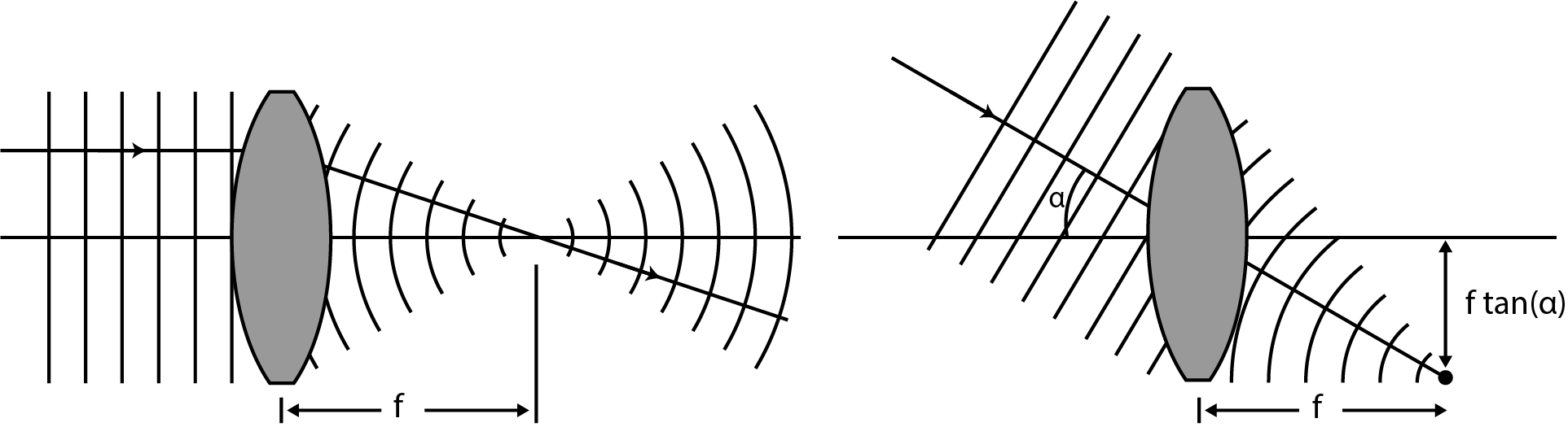
Figure 9:The course of the wavefronts at the focusing of a light bundle with a plane wavefront. On the right, the relation between the direction of the bundle and the position of the focal point is shown.
When the focal point is placed on a screen, the position of the spot can be used to determine the direction of the bundle. The relation between the direction of the bundle and the position on the screen is shown on the right side in Figure 9.
Incident light bundle. Optical system.
At the derivation of eq. (2) we assume that the incident light is a parallel bundle. This assumption is not justified for the lamp used in this experiment. The light of the mercury lamp is divergent by nature. To counter this, we will need to collimate the sources.
Collimation is easily done for a point source. You only need to place the source in the focal point of a convergent lens. In fact, the exact opposite of what is happening in Figure 9. Unfortunately, the lamp used in our experiment is not a point source. A small slit placed in the focal point of a lens will be needed to collimate the source, see Figure 10.
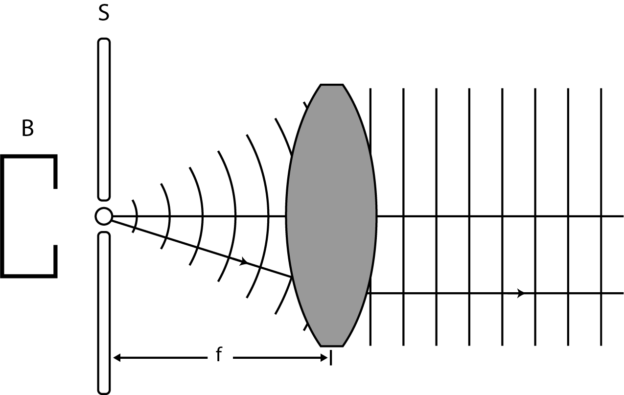
Figure 10:By placing the lens at the right position, the source is collimated.
The narrower the slit, the better the light from the lens can be characterised as one plane wave with one sharp direction. A disadvantage is of course that the intensity of the light that falls on the diffraction grating diminishes as the slit is narrowed.
Our setup for the determination of the wavelength of spectral lines with a diffraction grating now consists of: a source (lamp), a slit, a collimating lens, the diffraction grating, an image lens, and a screen. These parts will be setup in such a way that an image of the slit is formed on the screen.
What determines whether the size of the slit is reduced or magnified in the image? What is beneficial to the accuracy of the determination of the wavelength of a spectral line: a reduction or magnification? Explain.
Method
Setup
The setup that we will use for the determination of the wavelength of the visible spectral lines of the Hg lamp is shown in Figure 11. This setup is also called the monochromator setup. The only moving part of the setup is the diffraction grating. The grating will be mounted on a turntable with an angle distribution that makes it possible to measure the angle (See Figure 11).
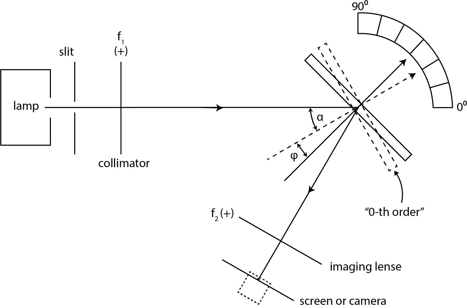
Figure 11:Setup for measuring the wavelength of spectral lines.
Using a slit directly behind the lamp, and a lens F produce a collimated (parallel) light bundle. This bundle hits the diffraction grating. We have seen that, because of the diffraction of the light through the grating, depending on the wavelength, parallel bundles are reflected at different angles. By changing the angle of the diffraction grating in respect to the incident light bundle, we can make a certain colour fall on a set point on the screen or the camera with the help of lens F. From the according angle, we can calculate the wavelength of the light.
At one specific angle for the diffraction grating, it seems like the light is conveyed. At this angle it seems like the light is portrayed by a normal mirror (via the lens F) to the set point on the screen. In fact, the 0 order diffraction pattern is portrayed in the set point. This does not change with the wavelength of the light. This position is shown in Figure 11 by the dotted line. The angle between the normal on the diffraction grating and the direction of the incident light is (thus the angle between the incident and reflected wave is 2). Note that is determined by the positions of the lamp, the lens F, the lens F, and the point on the screen.
If we want to use a certain setup in practice for, for example, the measurement of a number of spectral lines, then we measure the angle between the normal of the diffraction grating and the ‘mirror position’. In Figure 11 this angle is .
Elaboration
If we call the incident angle and the reflected angle , then the following formulas apply (see Figure 11)
In which is the number of lines per length unit, the wavelength and the order of diffraction . Note that can be either positive or negative.
For the situation drawn in Figure 11, is positive or negative? Does this correspond to your answer from question 5?
From measurements of and we can use eq. (4) to calculate . If we call the uncertainties in and , u() and u() respectively, derive the law of propagation of errors for the uncertainty in , .
If the difference between two spectral lines is very small, they cannot be distinguished by the naked eye, and the diffraction grating cannot be rotated accurately enough.
To still be able to measure the little wavelength difference, we replace the screen by a camera. The enlargement of the camera allows us to be able see and accurately measure the separation between the spectral lines.
The procedure for this is as follows. From the grating equation (2) follows that with a set angle of incidence i, a small change in the wavelength is paired with a small change in the angle of reflection . The relation is:
We calculate from the distance of the spectral lines on the camera and the focal point of f. The unit of is radian.
With eq. (5) we can determine from measurements of and . Of course you want to know uncertainty in . If you use the law of propagation for errors in the common way, you encounter a notation problem. Thus, call the angle of reflection v (was u) and the change in the angle of reflection (was ). If we indicate the uncertainties in v and with and , derive the law of propagation of errors for the uncertainty in , ).
Resolving (separating) power
Spectral lines have a certain width. It is clear that when the distance between two separate lines decreases, they will overlap and become indistinguishable from each other, at least with the naked eye. The intensity of the light as function of the wavelength is shown in Figure 12.
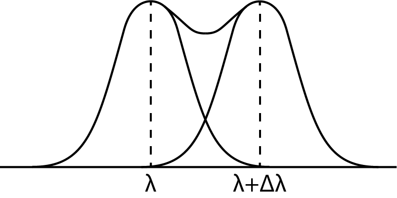
Figure 12:Resolving power
The resolving power of the setup is characterized by the quantity :
in which is the smallest observable difference in wavelength. This equation only holds for the first order. For higher orders we expect more spacing between spectral lines. Therefore the resolving power is higher at higher orders.
In practice, we make a prediction for based on a picture of two nearby spectral lines. We use this estimated value and the average value of the two spectral lines. We can compare this value with the theoretical upper limit:
in which is the order of the spectral lines. is the total number of grading lines involved in the interference process. If the entire grating is used, resembles the total number of lines of the grating.
Method
Preparation phase
First and foremost: visor trusts that you will use the equipment with care at the practicum. This applies especially to the handling with the diffraction gratings and lenses. Do not be clumsy! Read the following instructions and apply them!
ONLY HOLD THE DIFFRACTION GRATINGS AT THE RECTANGULAR FRAME OR AT THE STEM OF THE FRAME. A fingerprint or a scratch can not be cleaned or repaired. Diffraction gratings are very expensive.
The spectral lamps become hot when they are turned on. Only hold the stem of the lamp. Otherwise you can get burned badly.
Hold the lenses and other optical components at the stem of the frame.
Make sure that all components are tightly secured with the clamp and screw on the breadboard.
Again: Do not touch the lenses and diffraction gratings in the central part.
Do not leave equipment on the edge of the table. Secure them. Things can fall on the ground and break.
Do not leave components on the table. This way you prevent damage.
Do not look into the lamp directly. This can damage your eyes.
Turn the lamp, camera and computer off when you do not use them.
A tip: When setting up the experiments, you have to make sure that the entirety of the optical system is in line. Make sure that the elements that have to be in line, really do line up. Look at your setup from above and use the lines on the breadboard. Also make sure all elements are at the same height. Look from the side and use the height indicator.
Experimental phase
Build the monochromator setup. Use the Hg lamp and the 600 lines per mm diffraction grating. Start with the screen. Hold enough distance to be able to replace the screen by the camera. Control the collimation and assure yourself that the screen is in the focal point of f.
Rotate the diffraction grating such that . (use autocollimation, ask the assistant). Read the angle from the angle scale. This the zero point. Pick a point on the screen and rotate the diffraction grating such that the 0-th order falls exactly on that point. How do you recognise the 0-th order here? Read the angle scale and determine . Do not forget to estimate the uncertainty in the angle. Play around with the width of the slit.
Now rotate the diffraction grating systematically and notate the angle for each spectral line that falls on the chosen point on the screen. Do this for as many orders as possible. Make a table with the headings: colour, order, reading, , , u() and the result from preparation question 10. How do you get ? Use Python to help you fill in the last three columns. Also note that a set of colours represents one order.
Make a plot in which you plot the calculated wavelength on the vertical axis with its respected uncertainty against the order m on the horizontal axis. Plot the literary values as horizontal dotted lines in the same figure.
Calculate the weighted average of the wavelength for each measured spectral line and calculate the uncertainty in this average value. Take as weight . Use the given formulas from the Appendix for this. Does the result contradict the literary value?
Next, study the splitting of the yellow Hg lines. Replace the screen by the camera. Portray an order of the yellow lines on the camera (note: The colour can be different on the screen. Pay close attention.). (Think about the width of the slit and the use of the filter). Save the result for the report. (Use the save icon at the middle top.) Determine the distance between the lines on the screen in pixels. Calculate the difference in the angle of reflection from this. Check if your value of u is still current. Calculate the difference in the wavelength with eq. (5). What is the uncertainty ?
Replace the Hg-lamp with the Na-lamp and use the camera instead of the screen. Measure the angels of the visible spectral lines. What is the angle that corresponds with the 0 order? Specify the orders to the measured angles and calculate for each order the wavelength and its uncertainty. Again try to find splitting for all lines (except the 0 order of course). Do the individual results agree with the literature values? Calculate the weighted average and its uncertainty.
Evaluation phase
Determine the difference in wavelength of the two Na lines. Try to do this for all the orders. What is the associated uncertainty? At what order do you obtain the best results? Are the results in agreement with the literature values?
What is the smallest difference in wavelength that you can determine using this set up? What is the resolving power of this set up? What is the expected, theoretical value for the resolving power? What can be done to improve the results?
Finally Suggestions for the improvement of the experiment and the manual or ideas about what you would like to research with the used instruments, please mail to: c
Appendix
For the calculation of the weighted average you need to first calculate the weights, this is done in the following way:
This means that datapoints with a high uncertainty get a lower weight. And datapoints with a low uncertainty get a high weight (thus are more important). To find the final value for we use the following equation:
The final error/uncertainty in is equal to:
- Wolfson, R., & others. (2007). Essential university physics (Vol. 1). Addison-Wesley San Francisco, CA.