Falling waterdroplet - Introduction to Experimentation in Physics

Goal¶

What is the velocity of falling water droplets, how strong is the drag force exerted on these droplets by the surrounding air and what is their shape? These questions are addressed in this assignment. The primary goal of the experiment is to determine the drag coefficient, which is a measure for the drag force experienced by a falling water droplet in air.

Background¶

Introduction¶

Newton’s second law provides the equation of motion for a falling water droplet in air:

m\frac{dv}{dt}= mg - F_D - F_B

(1)

Here $m$ is the mass of the droplet, $v$ the velocity of the droplet, $g$ the gravitational acceleration, $F_D$ the drag force and $F_B$ the buoyant force. The velocity is defined relative to the stationary air, taking downward as positive. The drag force is the result of friction of the droplet with the air. The buoyant force is described by Archimedes’ principle.

In the rest of this manual $F_B$ is neglected. It can be expected that $F_D$ depends on the velocity of the droplet. In this experiment you will determine $F_D$ for a range of occurring velocities. To this end, you will perform two experiments:

with a drop test, you will determine the position-time relation of the falling droplet
with a visualization experiment you will take photographs of a floating droplet to determine its shape.

Falling droplet and fluid mechanics¶

It is generally assumed that the drag force $F_D$ is proportional to the velocity squared of the moving particle, in this case a water droplet:

F_D = \frac{1}{2}C_D A_{\perp}\rho_{air} v^2

(2)

Here $C_D$ is the drag coefficient, $A_{\perp}$ the cross-sectional area of the droplet perpendicular to the direction of the velocity and $\rho_{air}$ the air density. The value of $C_D$ , in turn, can also depend on the velocity. Furthermore, $C_D$ depends on the shape of the droplet.

In the field of transport phenomena, one often uses characteristic numbers (in Dutch: kentallen). These are dimensionless parameters that describe a system in a general way. The Reynolds number, Re, is the most important characteristic number in fluid mechanics. It is not only used to determine whether a flow is laminar or turbulent, but also to realize similarity between two different flows. The Reynolds number is defined as:

\mathrm{Re} = \frac{\rho v d}{\mu},

(3)

with $d$ is a characteristic dimension, here the largest diameter of the droplet perpendicular to the velocity, and $\mu$ the dynamic viscosity of air. Figure 1 gives the dependence of $C_D$ on the Re-number, for a spherical and a cylindrical particle.

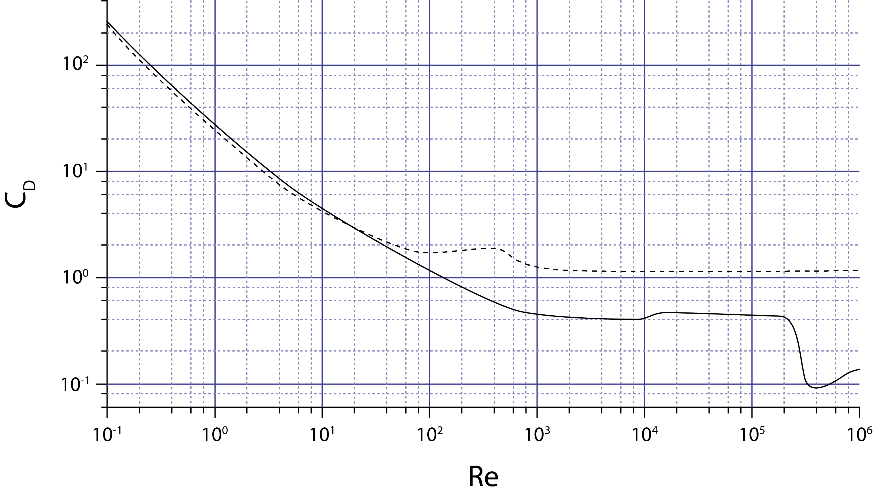
Drag coefficient C_D as a function of the Re-number, for a sphere (----) and a disk (- - -). — Figure 1:Drag coefficient $C_D$ as a function of the Re-number, for a sphere (----) and a disk (- - -).

For a low Re-number (Re $<$ 1) Stokes’ law applies:

F_D = 3\pi\mu d v

(4)

On the basis of the above, it follows for Re $<$ 1:

C_D = \frac{24}{\mathrm{Re}}

(5)

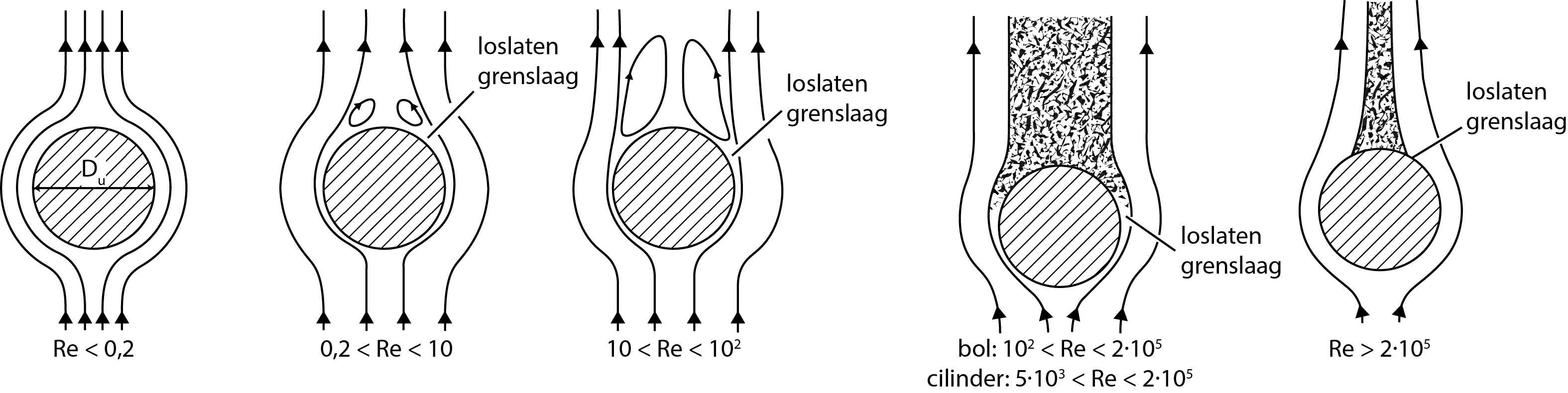
Figure 2:Flow pattern around a sphere as a function of the Re-number.

With increasing Re-number, vortices arise at the rear of the particle (see Figure 2). A wake is created; the boundary layer is “released” from the particle as a result of the inertia of the surrounding medium, that prefers to move straight on. N.b.: This line of reasoning assumes a medium flowing around the particle, but that situation turns out to be equivalent to the situation of the particle moving through the medium, as in the present experiment. For larger Re-numbers, the vortices increase in size and the location where the boundary layer is released moves to the front side of the particle. For even larger Re-numbers ( $10^3$ - $2\cdot 10^5$ , Newton regime) the wake becomes irregular and turbulent. Vortices are then carried along by the flow and new vortices are generated at the rear of the particle. Eventually, for very large Re-number, the boundary layer becomes turbulent and the location where the boundary layer is released moves back to the rear of the particle. In the transition range from the Stokes to the Newton regime, we can use the Schiller-Naumann relation:

C_D = \frac{24}{\text{Re}}(1+0.15\text{Re}^{0.687})

(6)

For objects moving with high velocity through a thin medium ( $10^3<\text{Re}<2\times10^5$ ), Figure 1 shows that $C_D$ is approximately constant.

Solution of the equation of motion¶

Using (2) and $\beta = C_D A \rho /2$ , (1) can be rewritten as follows:

m \frac{dv}{dt} = mg - \beta v^2

(7)

Here $F_B$ is neglected, as indicated earlier. This way of writing of the equation suggests that the parameter $\beta$ is constant. In that case the drag force would be proportional to the velocity squared. In general, however, this is not true, since $C_D$ yet depends on the Re-number (see Figure 1). Equation (7) is a non-linear (and therefore difficult to solve) differential equation in the velocity of the droplet. To illustrate the velocity behaviour, we have plotted in Figure 3 the exact solution of eq. (7) for a situation representative of this experiment. Herein, it has been taken into account that $\beta$ depends on the velocity, through $C_D$ . This solution has been obtained using numerical methods. In the Figure it can be seen that the droplet after approximately four seconds almost reaches its saturation velocity of 12.9 m/s. This exactly equals the value $v_{sat}=\sqrt{mg/\beta}$ following from Eq. (7) for $C_D=0.4$ . As will become clear, the maximum drop time in the experiment is about 0.6 s. Thus, the saturation velocity is far from reached.

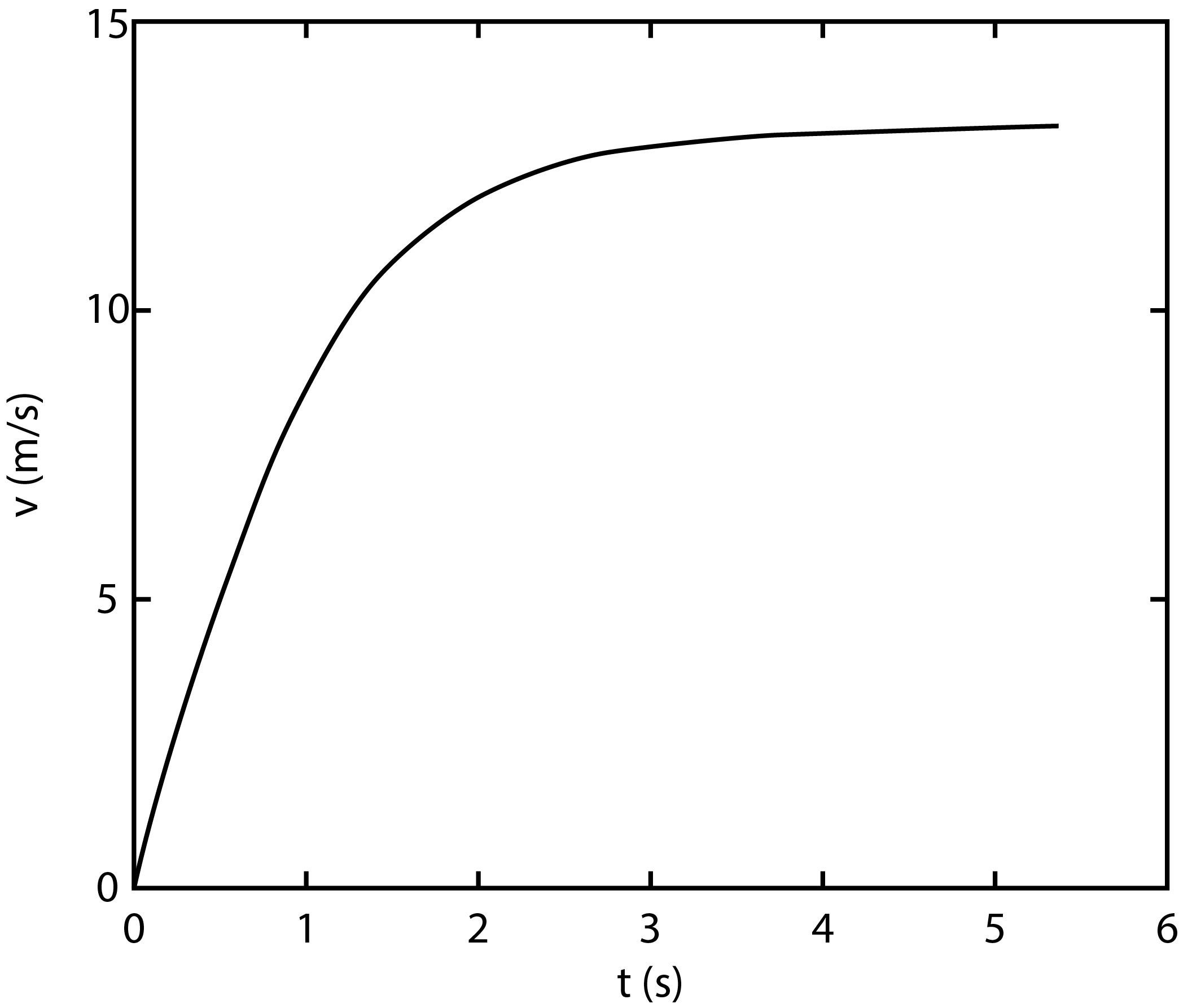
The velocity of a falling water droplet in air as a function of the drop time. The diameter of the droplet, taken here as spherical, is 6 mm. After about 4 s, the saturation velocity is almost reached. The curve is the exact solution, obtained by numeric integration of Eq. . — Figure 3:The velocity of a falling water droplet in air as a function of the drop time. The diameter of the droplet, taken here as spherical, is 6 mm. After about 4 $s$ , the saturation velocity is almost reached. The curve is the exact solution, obtained by numeric integration of Eq. (7).

An approximate solution of Eq. (7), satisfying the present goal, can be obtained in the following globally sketched way. Integration of Eq. (7) gives

v(t) = gt - \frac{1}{m}\int_{0}^{t} \beta (v(t'))v(t')^2 \mathrm{d}t.

(8)

This did not help much yet, as we have expressed $v(t)$ as an integral of the function $v(t)$ , and that is just the quantity we are looking for. However, by repeated substitution of the expression for $v(t)$ “in itself” and by assuming that $\beta$ is time-independent, the following approximation for the drop velocity $v(t)$ is found:

v(t) = v_0 + gt - \frac{1}{3}\frac{\beta}{m}g^2t^3 + \frac{2}{15}\left(\frac{\beta}{m}\right)^2 g^3t^5 + ...

(9)

The four terms in the expression for $v(t)$ are the initial velocity, the free drop term, the first order correction and the second order correction, respectively. From further theory, it follows that for this experiment the first order correction is sufficient, provided $t < 0.7$ s. In that case, the second order correction is negligibly small compared to the first order correction. It turns out that the this condition for the drop time is met in the experiment.

In Figure 4 curves for the drop velocity and the drop distance have been plotted, indicating the error with respect to the exact solution if only the first order term in Eq. (9) is included. In this, for the first order term $C_D=0.4$ has been taken, the constant value for a spherical droplet also used for Figure 1. Given the maximum drop time of about 0.6 s, the error is less than 1% for the drop velocity and less that 0.3% for the drop distance. In this experiment we neglect these errors. Note that the larger values of $C_D$ , occurring for the smaller velocities at the start of the drop trajectory, apparently do not play a significant role.

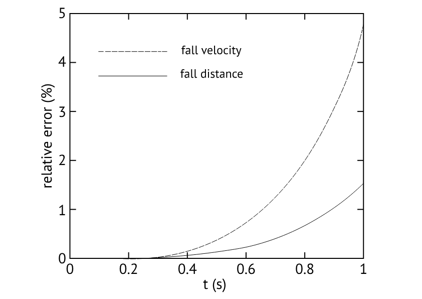
Figure 4:The relative error in the drop velocity and the drop distance of the water droplet with respect to the exact result, when only taking into account the effect of the drag force to first order. The diameter of the spherical droplet is 6 mm for both curves.

Experimental approach¶

Integration of Eq. (9) with neglect of the second order correction leads to

s(t) = s_0 + v_0t + \frac{1}{2}gt^2 - \frac{\beta g^2}{12m}t^4

(10)

where $s_0$ is the travelled distance at $t=0$ . When we design the experiment such that at $t=0$ both the traveled distance and the velocity are zero, then eq. (10) reduces to

s(t) - \frac{1}{2}gt^2 = -\frac{\beta g^2}{12m}t^4

(11)

In words, this says that the drop distance in air at any time is reduced with respect to the drop distance of a free fall by an amount proportional to the drop time to the fourth power. The proportionality constant includes the parameter $\beta$ , which in turn is proportional to $C_D$ . This result immediately suggests the experimental approach: for various drop distances $s_i$ measure the corresponding drop times $t_i$ $(i=1,2,3,...,n)$ and put the measured data points in a plot with the quantity $\Delta=s(t)-gt^2/2$ on the vertical axis and $t^4$ on the horizontal axis. A linear fit to the data points then has the slope $-\beta g^2/(12m)$ . Since we have $\beta=\rho_{air} A_{\perp} C_D/2$ , $C_D$ can be determined from the slope, provided that $m$ and $A_{\perp}$ are known. The mass $m$ is determined through weighing, while the perpendicular area $A_{\perp}$ is determined in a visualization experiment of a floating water droplet (see the next paragraph).

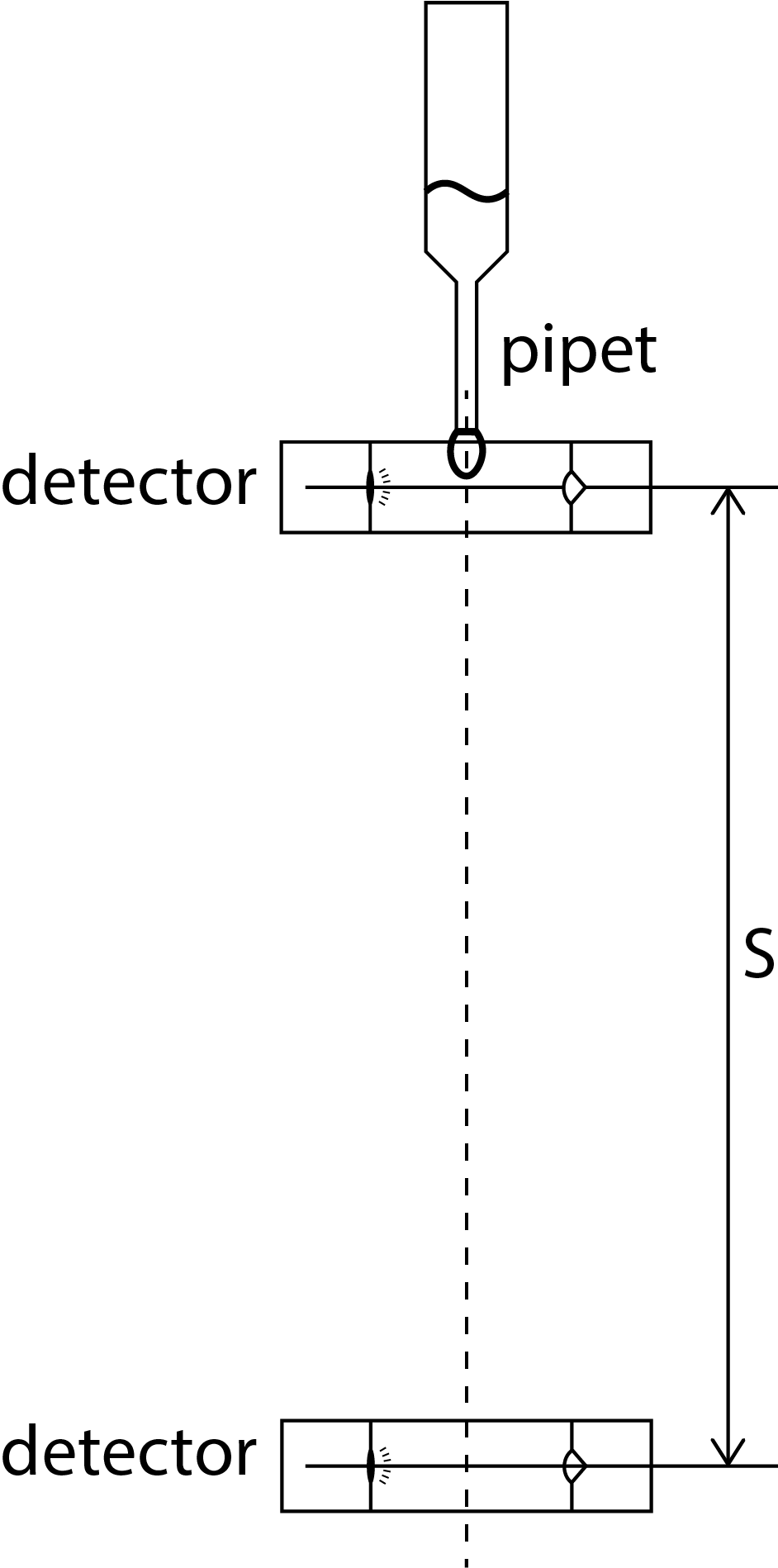
Schematic of the drop test. The droplet falls a distance s. — Figure 5:Schematic of the drop test. The droplet falls a distance $s$ .

Figure 5 gives a sketch of the setup. Using a pipette, you will make a droplet, which is released once it is big enough. With two optical detectors you will measure the time $t$ it takes for the droplet to fall $s$ meter. The drop distance $s$ equals the distance between the two detectors. The first detector is located at $s = 0$ , as close as possible to the point where the droplet is released from the pipette. The position of the second detector can be varied. The detectors consist of a laser and a photodiode, together forming a light gate. When a droplet passes a light gate, the laser beam is briefly interrupted, causing a pulse in the signal of the photodiode. A counter connected to the light gates measures the time difference between the two pulses, i.e. the drop time $t$ .

Visualization experiment¶

When you ask somebody to draw a droplet, it is very likely that the person asked will draw the shape of a tear: thick at the bottom and converging to a tip at the top. A falling water droplet, however, is rather flat than elongated. A falling droplet resembles an “M&M”. To establish the shape of a droplet that is subject to air drag and to determine its cross-sectional area $A_{\perp}$ , and from this the drag coefficient $C_D$ , you will take photographs of the droplet. To enable this, you will float the droplet by placing it in an upward air flow in the setup depicted in Figure 6.

Position the pipette a few centimeters above the wire mesh, with the blower set to about 20 Volt, and create a droplet. Try to keep the floating droplet stable in the air flow long enough to take sharp photographs. This requires some trial and error and optimization with (among other things) the blower voltage and the pipette’s position relative to the mesh. A transparent cylinder is available to guide the air flow, if necessary. Dry the mesh with a tissue if a droplet has fallen onto it; otherwise the setup is not ready for the next attempt.

While floating a droplet, it is difficult to press the camera button and at the same time keep the camera setup stable. Therefore, use the camera’s remote control to take the photographs. Take quite a number of photographs and view them on your laptop or on a computer of the laboratory course.

Determine the cross section and volume of the droplet. Determine the droplet’s absolute dimensions using an object of known size in the photograph. The floating droplet is heavier that the falling droplet, but we suppose that its shape is the same. Beware: after the experiment, all data on the memory card of the camera will be deleted. Therefore, copy photos to a memory stick or to your laptop. Otherwise, you will not have a photograph for your report.

Assignments¶

For the formulation of the problem see chapter 1, GOAL, and chapter 2, section 2.1. A separate afternoon has been scheduled for the problem analysis and setting up the measurement plan.

Do the following assignments.

Exercise 1

Find literature values for $g$ , $\rho$ and $\mu$ .
Prove with a calculation that the buoyant force can indeed be neglected.
Derive eq. (5).
The upper detector is positioned such that the droplet will be detected immediately after release, meaning this detector does not require any adjustment. Position the lower detector as low as possible. Subsequently, you can vertically align the setup with a plump line. Perform the alignment and “lock” this by carefully raising the plateau of the lab jack, so as to make it touch the bottom of the tube with gentle but sufficient force. For proper alignment, a large fraction of the droplets will be detected and will result in the correct drop time on the display of measuring device.
Determine the uncertainty in $s$ and $t$ .
Find a way to measure the mass of a droplet. Practice generating droplets and judge your skill from the width of the mass distribution of generated droplets (histogram). How does the measured standard deviation of the droplet mass compare to the uncertainty of a reading with the Mettler Toledo balance (0.1 mg)? What is your final estimate for the uncertainty of the mass of the droplets used in the drop tests and how did you obtain it?
Find out how the camera and remote control work.
Find out what information can be obtained from the photograph of the droplet, and how you can determine a scaling factor to correct for the difference between the falling and floating droplet. The scaling factor $\alpha$ is defined by relating the volume the falling droplet to that of the floating droplet: $V_{fall}=\alpha^3 V_{float}$ . This translates to $m_{fall}=\alpha^3 \rho_w \frac{1}{6} \pi D^2 h$ . Herein $m_{fall}$ is the mass of the falling droplet and $\rho_w$ the density of water. $D$ and $h$ are the long and short axis of the ellipse visible in the photograph of the droplet, respectively.
Why is the floating droplet heavier than the falling one, and why are their shapes identical?
Determine the uncertainty in $A_{\perp}$ . For this use $A_{\perp}=\frac{1}{4} \pi (\alpha D)^2$ .
Express the drag coefficient $C_D$ in quantities you have measured or obtained otherwise, and derive the equation for the uncertainty of $C_D$ .
Make an estimate of the (range of the) literature value of $C_D$ , use Figure 1 for this.

Set up a measurement plan and discuss this with the teaching assistant (TA). After approval by the TA, execute the plan on the scheduled afternoon.

Determine the drop time for at least 10 positions of the lower detector. The lower detector cannot be positioned above the edge of the table. Handle the setup very carefully and calmly, to prevent that you have to re-align it.

Use Python for the data processing. Ask the TA for help, if necessary.

Write a report on the experiment, according to the guidelines of the Physics Laboratory Course. The deadline for handing in the report and the lab journal is known at the administration of the Physics Laboratory, room A001.

Addendum taking a picture¶

To take a good picture of the droplet, light is required. It must be really bright as the droplet is still moving and you get only a good picture if the shutter speed is really high. To obtain a useful picture without wasting much time, we should make the decisions rather than the camera. The camera is therefore set to manual with a shutter speed of 1/320 s, a diafragma of f9, and an ISO value of 400. The flashlight is turned off.

Setting the camera to manual also requires a manual focus. Choose the largest focal distance possible (55mm) and focus on the tip of the needle of the pipet. Move the camera as close as possible towards the setup. Focussing should still be possible.

By taking the picture from a small angle, you will have a light spot from one of the lamps in the background. This gives an excellent contrast to determine the circumference of the drop. Keeping the shutter release button pressed while letting the pipette drip gently gives the best chance of a usable image. Note that the drop may come towards or float away from the camera. If so, the pipette needle is in focus sharp. However, the water droplet will be out of focus. This will contribute to the measurement uncertainty.

First experiment

Spectral lines of Hg and Na

First experiment

Millikan