02 Fraunhofer and Fresnel Diffraction

Aim¶

To show how light illuminating a slit gives different regions of diffraction. Close to the slit: Fresnel diffraction and at some distance: Fraunhofer diffraction. To determine where the one type of diffraction transforms into the other.

Subjects¶

• 6C20 (Diffraction Around Objects)

Diagram¶

Equipment¶

• Magnetic clamps, used to fix the components to the steel table.

• Laser, $50 \mathrm{~mW}$.

• Two surface mirrors ( $1 / 10 \lambda$ ).

• Lens, $\mathrm{f}=+10 \mathrm{~mm}$.

• Lens, $\mathrm{f}=+50 \mathrm{~mm}$.

• Adjustable diaphragm.

• Slide holder.

• Lens, $\mathrm{f}=132 \mathrm{~mm}$.

• Optical rail, $\mathrm{I}=1 \mathrm{~m}$, as guiding ruler.

• Adjustable slit.

• Video camera.

• Projector to project diffraction-image.

• Overheadsheet with Figure 10.5 (“Optics” by Hecht; see Sources).

Presentation¶

Preparation¶

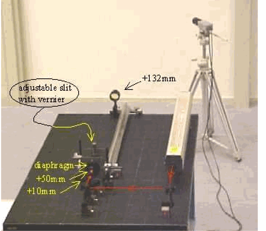
The demonstration is set up as shown in Diagram:

-The two mirrors are positioned in such a way that the laserbeam passes parallel to the table.

• The two lenses ( $+10 \mathrm{~mm}$ and $+50 \mathrm{~mm}$ ) are positioned at an intermediate distance of $60 \mathrm{~mm}$. Having passed these lenses, the laserbeam is broadened. Take care that the broadened beam is still parallel to the table.

-The lens of $132 \mathrm{~mm}$ can easily be shifted in this beam up and down using the carefully positioned guidance rail.

Demonstration¶

The set-up as described in “Preparation” is explained to the students, so that it is clear to them that the adjustable slit is placed in a beam of light consisting of parallel rays. The adjustable slit is set at $.6 \mathrm{~mm}$. The $+132 \mathrm{~mm}$ lens is shifted close to this slit to project a sharp image of it on the wall: a smooth red region, having a sharp boundary on both sides (see Figure 2A). Considering the wall to be far away, the lens needs to be $+132 \mathrm{~mm}$ away from the slit (the slit is in the focus of the projecting lens).

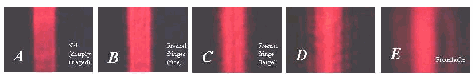
Then the $+132 \mathrm{~mm}$ lens is slowly shifted away from the slit. The projected image changes: in the originally smooth red region domains of higher and lower intensity (fringes) can be discerned (see Figure 2B). Moving out still farther, the fringe pattern changes continuously: the number of fringes diminishes while the fringes themselves broaden (compare the pictures in Figure 2; reality is better than the quality of these pictures). When the $+132 \mathrm{~mm}$ lens has reached the end of the guidance rail the familiar diffraction pattern as shown when introducing diffraction, is visible (see the demonstration “Diffraction(2), single slit”).

Leaving the $+132 \mathrm{~mm}$ lens in this far away position, the transformation from Fresnel to Fraunhofer can also be shown when you vary the width of the slit.

It will be clear now that distance form the slit and slit-width have both something to do with this transformation of one type of diffraction into the other.

Explanation¶

The $+132 \mathrm{~mm}$ lens being for away from the wall projects an image of an “object” that is $132 \mathrm{~mm}$ away form it. At first we seen the sharply imaged slit; moving away from the slit, for instance $10 \mathrm{~mm}$, then the image of this position is projected on the wall. In this way the lens scans the region close to the slit (near field) and farther away (far field). Considering far field diffraction (Fraunhofer diffraction) the slit is that narrow compared to the distance in the field, that the secondary wavelets emerging from the slit proceed as being planar. This relative simplicity of Fraunhofer diffraction is explained in the demonstration “Diffraction(2), single slit” in this database.

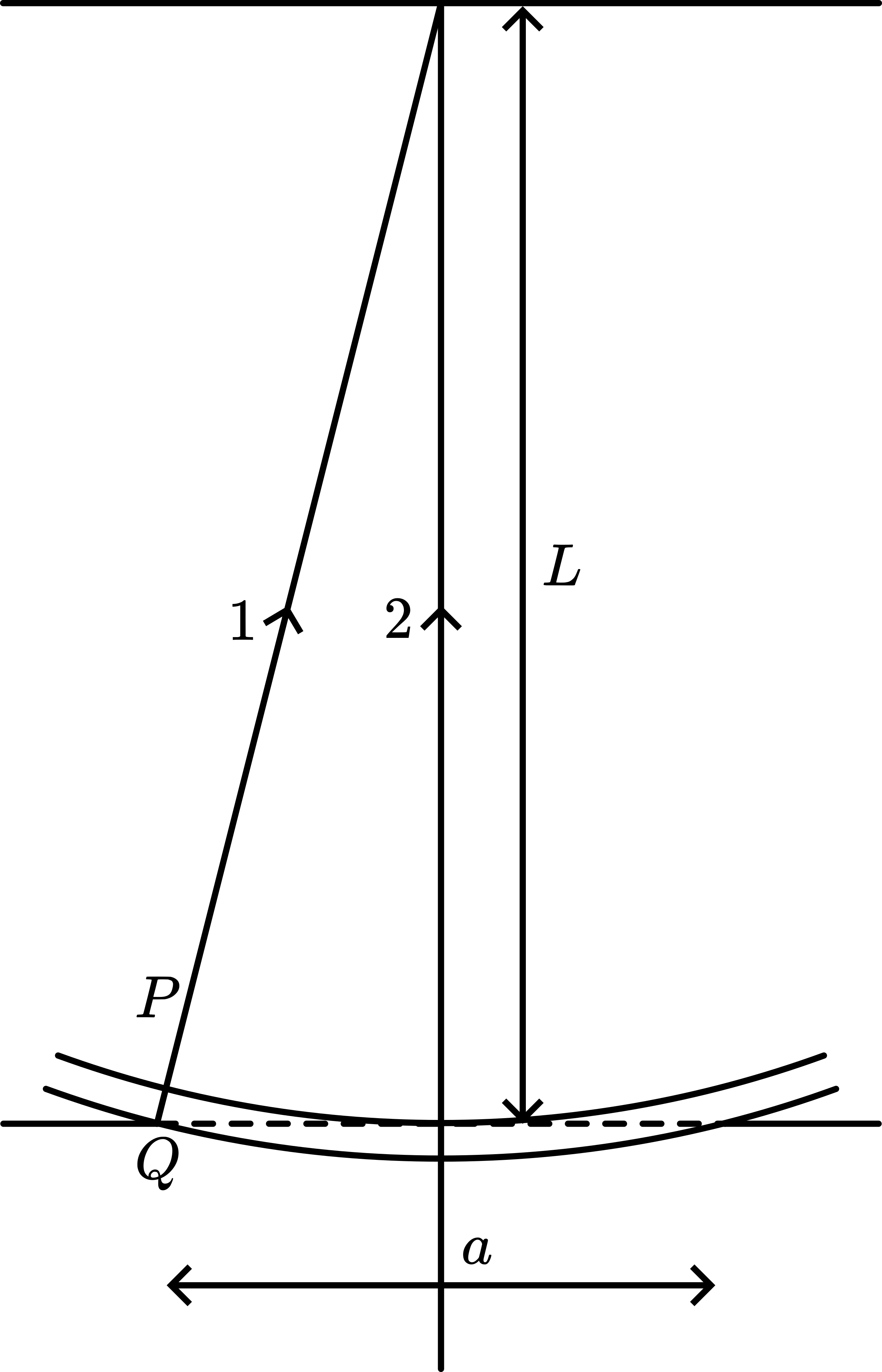
In the near field configuration the width of the slit cannot longer be neglected. Due to this an extra path difference (PQ) between ray 1 and ray 2 is introduced (see Figure 3).

Applying Pythagoras shows $L^{2}+\frac{a^{2}}{4}=(L+P Q)^{2}$, and $P Q=\frac{a^{2}}{8 L}$. If, as a rule of thumb, this extra path difference is neglected if it is smaller than $\lambda / 4$, we find that for the distance $L$ we need $L>\frac{a^{2}}{2 \lambda}$. So, the distance $L \approx \frac{a^{2}}{2 \lambda}$ can be considered as the “border” between Fresnel - and Fraunhofer diffraction. Applying the data In this demonstration $(a=.6 \mathrm{~mm} ; \lambda=650 \mathrm{~nm})$, we find: $L=.25 \mathrm{~m}$. Performing the demonstration confirms this.

Remarks¶

• In preparing this demonstration we used of course $L=.25 \mathrm{~m}$ (means: lens at $.382 \mathrm{~m}$ from slit) and then calculated the needed slit width, so that both types of diffraction can be clearly shown in one shift of the $+132 \mathrm{~mm}$ lens.

• The demonstration can also be performed having the $+132 \mathrm{~mm}$ lens fixed at the end of the table $(L=.85 \mathrm{~m})$ and then slowly increase the width of the slit. Then the distinction between Fresnel - and Fraunhofer diffraction is at a slit width of around $1 \mathrm{~mm}$. But realize that turning a vernier is less visible to an audience than shifting a lens across the table.

• The different patterns can also be registered using a pattern scanner as described in [“Diffraction(1), introduction”](../../6C20 Diffraction Around Objects/6C2001 Diffraction introduction/6C2001.md>) in this database. Particularly the fine fringes close to the slit can be made visible in this way.

Sources¶

• Hecht, Eugene, Optics, pag. 437-438 and 495-499