6. Labjournaal#
6.1. General#
Template for labjournaal. See https://jupyter-notebook.readthedocs.io/en/stable/examples/Notebook/Working With Markdown Cells.html for options to use markdown.
#import necessary libraries
import matplotlib.pyplot as plt
import numpy as np
import math
from scipy.optimize import curve_fit
Names:
Title of the experiment: Validation of the relation between force and distance of two magnets.
Starting date:
Expected enddate:
Goal of the experiment: In this experiment we determine the relation of the force between two magnets as function of their mutual distance. We use the set up shown below:
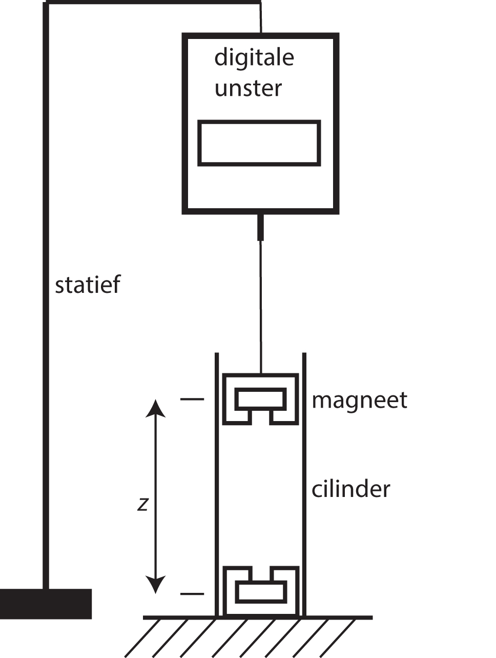
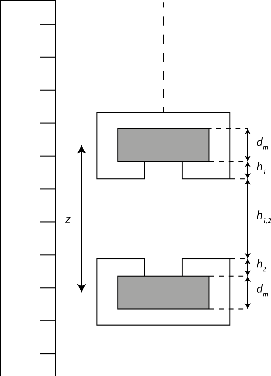
The heart to heart distance between the two magnets can be calculated:
Research question:
Expectations or Hypothesis:
Desired accuracy:
6.2. Preparation#
Assignments:
Method:
Theory:
Independent variable:
Dependent variable:
Controlled variablen:
Measurement instruments & Settings:
#Metingen vooraf
d_m =
u_d_m =

h_1_aan =
u_h_1_aan =

h_1_af =
u_h_1_af =

h_2 =
u_h_2 =
Procedure:
Setup(drawing or picture):
Notes:
About accuracy:
6.3. Execution#
# Measurements: Explain the names of variables provide only raw data in np.arrays!
#Raw measurements
# Note, these can be read in using the CSV file as well.
h_12_af = np.array([   ,   ,  ,\
                       ,   ,  ,\
                       ,   ,  ,\
                       ,   ,  ,\])

F_af =    np.array([   ,   ,  ,\
                       ,   ,  ,\
                       ,   ,  ,\
                       ,   ,  ,\])*9.81

h_12_aan = np.array([   ,   ,  ,\
                        ,   ,  ,\
                        ,   ,  ,\
                        ,   ,  ,\])

F_aan =    np.array([   ,   ,  ,\
                        ,   ,  ,\
                        ,   ,  ,\
                        ,   ,  ,\])*9.81
Observations:
Notes:
6.4. Processing#
Description of processing of raw data into scientific evidence:
z_aan =

z_af =
6.4.1. Data processing and analysis:#
First look at your data without considering measurements uncertainty. Use the next cell to insert your code to plot your measurements. Consider the rules producing graphs!
#Data processing and analysis:
#(F,z)-plot
plt.figure()
**[your code]**
plt.show()
Based on the plot, are you allowed to combined the two datasets into one? If so, merge the arrays.
#merge arrays
z =
F =
Now plot the same measurements with errorbars. You can use this source to find out additional options: https://matplotlib.org/3.1.1/api/_as_gen/matplotlib.pyplot.errorbar.html
#Data processing and analysis:
#(F,z)-plot with errorbars
plt.figure()
**[your code]**
plt.show()
6.5. Fitting the data#
6.5.1. function fit using \(z^{-4}\)#
There are at least two options to use a function fit to your measurements. We will look at the different methods to analyse your data below.
As we expect the function to be in the form: \( F = \frac{a}{z^4} \) we can ask Python to fit this function. You can use this source to find out additional options: https://docs.scipy.org/doc/scipy/reference/generated/scipy.optimize.curve_fit.html Think about whether measurements with the outcome \(F\) = 0 N count or should be disregarded.
def func(x,a):
	return a/x**4

popt,pcov = curve_fit(func,z,F)
print('alpha = ', popt[0], '+/-', np.sqrt(pcov[0,0]))
The printed value is the constant in the function \( F = \frac{a}{z^4} \). Make a new plot in which you show your measurements and your function fit. Part of the code is already written for you.
#(F,z)-plot with errorbars and functionfit
plt.figure()


**[your code]**

min_value_z =
max_value_z =

x = np.linspace(min_value_z,max_value_z,1000)
y = func(x,*popt)

plt.plot(x,y,'r--',linewidth=1)
plt.show()
6.5.1.1. Residual analysis#
It is always interesting to see whether the fit is a good fit. The fit above might not be the easiest way to directly see this. We therefor use a residual analysis. In this analysis we plot our measurements - our fit. The code gives some idea of what to do. Analyse the residuals by completing the code below.
# Residual analysis
plt.figure()
plt.plot(z,func(z,popt[0])-F,'k.',linewidth=1)
plt.show()
6.5.1.2. fitting with systematic error#
You were able to measure the heart-to-heart distance with a certain accuracy. You probable had to use some kind of reference point. Using a reference might lead to a systematic error. A systematic error can be introduced by looking at the function \(F=\frac{a}{(z+\Delta z)^4}\), where \(\Delta z\) is our systematic error. Investigate whether there is a systematic error in your data.
6.5.2. linear fit#
Another option is a linear fit. As we expect the function to be in the form: \( F = \frac{a}{z^4} \) we can replace \( z^{-4} \) by \( u \). Our function will then be a linear function: \( F = a \cdot u \). This is known as coordinate transformation and is already taught at secondary school level (so you should have some experience with it!).
Make a new variable \( u \) with the values of \( z^{-4} \) and plot the graph. Make it an interactive plot (%matplotlib notebook) where you can zoom in on certain parts of the graph. Does it look linear to you?
#(F,u)-plot without errorbars
plt.figure()
u =
**[your code]**
plt.show()
The errorbars are still missing in the plot. As \( u = z^{-4} \), \( u_u = 4 \cdot u_z \cdot z^{-5} \).
Proof this.
Calculate the uncertainties for \( u \) and errorbarplot (\( F \), \( u \)).
#(F,z)-plot with errorbars
plt.figure()
**[your code]**
plt.show()
Carry out the following steps:
define the function for the functionfit
curve fit
plot your measurements and the curve fit
make it an interactive plot so that you can zoom in and see all essential features of the graph
#(F,z)-plot with errorbars and functionfit
plt.figure()
**[your code]**
plt.show()
Make additional plots that are relevant for the experiment in the given context.
#additional plots of interest
plt.figure()
**[your code]**
plt.show()
There is at least one additional way to see what kind of exponential function (\( y = a*x^n \)) is used. One can use a log-log-plot to see whether n = -4 and constant! Explore this way of analyzing the data.
#extra analysis
plt.figure()
**[your code]**
plt.show()
Maybe you are not satisfied with the result… find out whether there is a different relation than \( F = \frac{a}{z^4} \) that better matches your experimental data, e.g. \(F = a \cdot z^{n}\)…
6.6. Calculating the remanent field#
If your data concords with the formula: \(F=\frac{\alpha}{z^4}\), we still have to see whether the remanent field is similar to the value specified by the manufacturer. This analysis consists of the following steps:
produce the value of \(\alpha\) and its associated uncertainty
using this value, calculate the remanent field \(B_r\)
calculate the associated uncertainty
produce an agreement analysis (strijdigheidsanalyse) to see whether the values are in agreement.
Execute this analysis.
Describing the pattern in the processed data:
#Calculations of e.a. measurement uncertainties, and providing final answers.
Notes: