03 Diffraction (2b), Single Slit#
Aim#
To show diffraction on a variable single slit.
Subjects#
6C20 (Diffraction Around Objects)
Diagram#
Fig. 602 .#
Equipment#
Steel table.
Magnetic clamps, used to fix the components to the steel table.
Laser, \(50 \mathrm{~mW}\).
Two surface mirrors \((1 / 10 \lambda\) ).
Lens, \(\mathrm{f}=+10 \mathrm{~mm}\).
Lens, \(\mathrm{f}=+50 \mathrm{~mm}\).
Adjustable diaphragm.
Slide holder.
Lens, \(\mathrm{f}=132 \mathrm{~mm}\).
Opticail rail, \(\mathrm{I}=1 \mathrm{~m}\), as guiding ruler.
Variable slit with vernier adjustment.
Overheadsheet with Figure 603.
Presentation#
Preparation#
The demonstration is set up as shown in Diagram:
-The two mirrors are positioned in such a way that the laserbeam passes parallel to the table. -The two lenses ( \(+10 \mathrm{~mm}\) and \(+50 \mathrm{~mm}\) ) are positioned at an intermediate distance of \(60 \mathrm{~mm}\). Having passed these lenses, the laserbeam is broadened. Take care that the broadened beam is still parallel to the table.
-The lens of \(132 \mathrm{~mm}\) can easily be shifted in this beam up and down using the carefully positioned guidance rail.
Demonstration#
The set-up as described in Preparation is shortly explained to the students. The most important in this explanation is that the slit will be placed in a broadened beam and that the adjustable slit will be illuminated by plane waves.
The laser is switched on. A spot of \(2 \mathrm{~cm}\) projects on the wall (see [“Diffraction(2a)](../6C2002 Diffraction Single Slit/6C2002.md>)). The \(+132 \mathrm{~mm}\)-lens is placed at the end of the guiding ruler, to project an enlarged image of the interference-pattern as it will be “seen” around \(85 \mathrm{~cm}\) (1m-132mm) behind the slit. The broadened and enlarged beam projects as a spot on the wall (diameter of the spot is around \(40 \mathrm{~cm}\) ). The slit is closed and positioned in the beam. (By means of an overheadsheet it is shown to the students what the geometrical projection will show to us (see Figure 603): When the wall is at a distance as indicated in this figure, then the slit width \(a\) is projected 20 times larger on the wall. So when the slit width is \(0,1 \mathrm{~mm}\), then we will see a width of \(2 \mathrm{~mm}\).)
Fig. 603 .#
-slit at \(0.2 \mathrm{~mm}\), band of light \(=15 \mathrm{~cm}\), first subsidiary maxima appear;
-slit at \(0.3 \mathrm{~mm}\), central band of light \(=8 \mathrm{~cm}\), four subsidiary maxima on both sides;
-further opening of slit compresses the observed diffraction pattern;
-slit at \(0.7 \mathrm{~mm}\), central band of light \(=1 \mathrm{~cm}\), around 10 subsidiary maxima on both sides (see Diagram C; reality is much better than this photograph).
At this \(0.7 \mathrm{~mm}\) slit width the first subsidiary maxima are almost as intens as the central maximum. Usually here we stop the demonstration (see Remarks).
Explanation#
When the slit is \(0.1 \mathrm{~mm}\) and the geometrical projection would be only \(2 \mathrm{~mm}\) wide, clearly light is bending, broadening the band to \(20 \mathrm{~cm}\).
Many textbooks give a detailed explanation (see Sources). We consider Figure 604.
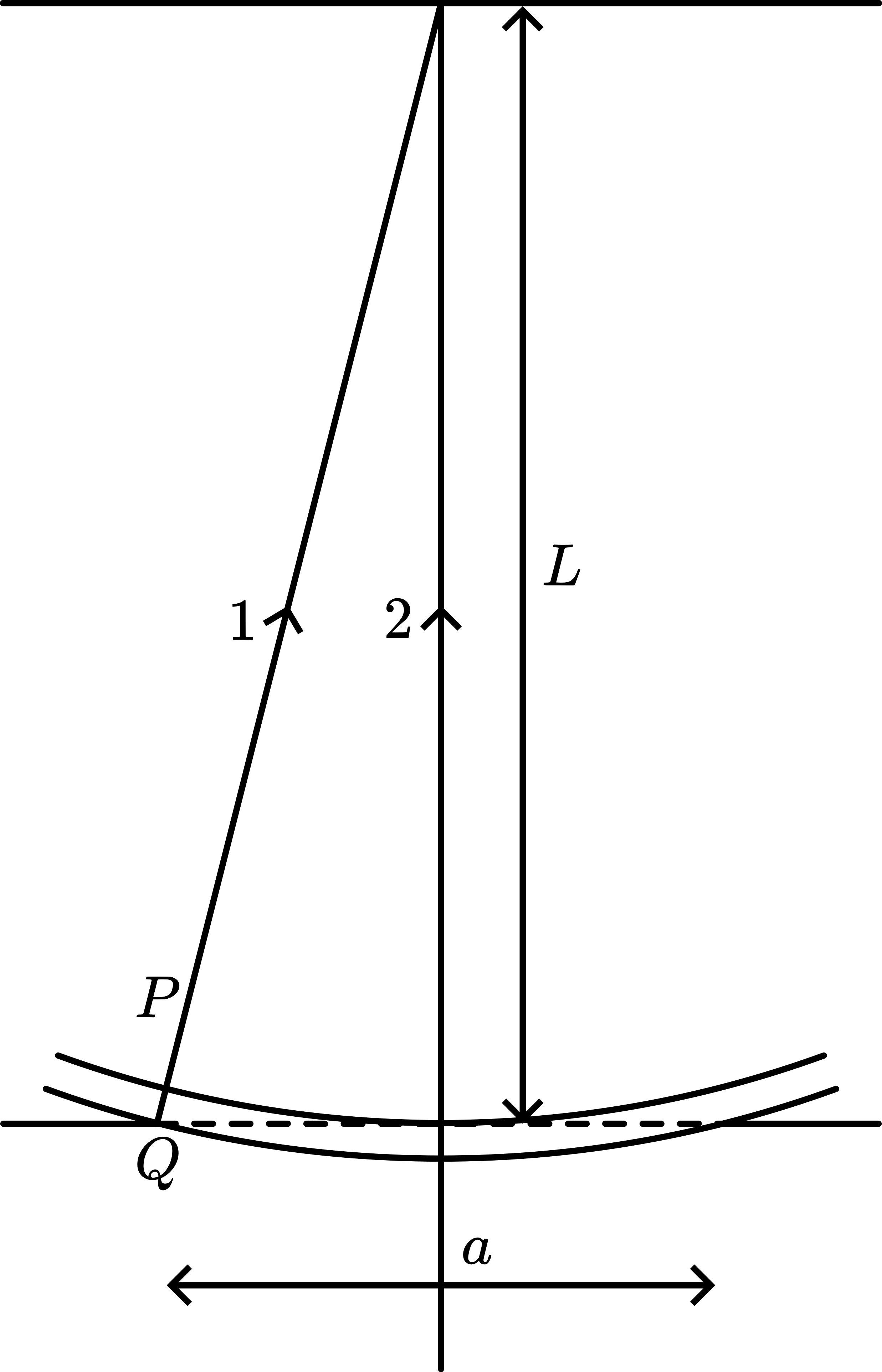
Fig. 604 .#
At \(\mathrm{P}, \mathrm{N}\) secondary wavelets superimpose, having a path difference of \(\frac{a}{N} \sin \theta\). Applying phase addition (see Figure 604B), \(\mathrm{A}_{p}\) is the resultant wave amplitude at \(\mathrm{P}\). At \(\mathrm{O}\), the total amplitude of the secondary wavelets will be the arclength in that phasor diagram, since all vectors then have the same phase. At Q ( \(\theta\) is larger) the phase difference between the “individual” secondary wavelets is larger and the phase diagram (Figure 604C) shows that the total amplitude can eventually be zero.
Analysis gives for the intensities \(\left(I_{\theta}\right)\) (see textbooks): \(\frac{I_{\theta}}{I_{0}}=\left[\frac{\sin \left(\frac{\pi a \sin \theta}{\lambda}\right)}{\frac{\pi a \sin \theta}{\lambda}}\right]^{2}=\left[\frac{\sin \alpha}{\alpha}\right]\). Minima occur at \(\sin \alpha=0\), so when \(\alpha=\mathrm{n} \pi\), and maxima at \(\alpha=\left(\frac{2 n+1}{2}\right) \pi\). The intensities of these maxima are then given by \(\frac{I_{\theta}}{I_{0}}=\frac{\sin ^{2} \alpha}{\alpha}=\frac{4}{(2 n+1)^{2} \pi^{2}}\).
\(\mathrm{n}=1\) gives \(\mathrm{I}_{1}=0.045 \mathrm{I}_{0}\);
\(\mathrm{n}=2, \mathrm{I}_{2}=0.016 \mathrm{I}_{0}\), etc.
So, the subsidiary maxima are comparatively weak, but yet clearly visible as the demonstration showed.
Remarks#
The \(+132 \mathrm{~mm}\) lens is positioned at a distance of about \(1 \mathrm{~m}\) away from the slit. This means that on the wall an image is projected of a point around \(85 \mathrm{~cm}\) (1m-132mm) away from that slit. In that way it is assured that the diffraction pattern is far field Fraunhofer pattern. Increasing the slit opening beyond \(0.7 \mathrm{~mm}\) will transfer the projected pattern into a Fresnel diffraction pattern, spoiling (complicating) our demonstration. The transition form Fraunhofer to Fresnel diffraction occurs in this set-up at around (see Figure 603): \(s=a^{2} / 2 \lambda, s=85 \mathrm{~cm}\), so \(a=1 \mathrm{~mm}\). In this single slit introductory demonstration we should not go beyond that width. (See the demonstration “Fraunhofer-Fresneldiffraction”.)
Sources#
Hecht, Eugene, Optics, pag. 442-447
Mansfield, M and O’Sullivan, C., Understanding physics, pag. 325-327
Young, H.D. and Freeman, R.A., University Physics, pag. 1167-1169
Giancoli, D.G., Physics for scientists and engineers with modern physics, pag. 890-893