02 Damped Galvanometer#
Aim#
To show various modes of damping (under-, critical- and overdamping)
Subjects#
3A50 (Damped Oscillators)
5K10 (Induced Currents and Forces)
Diagram#
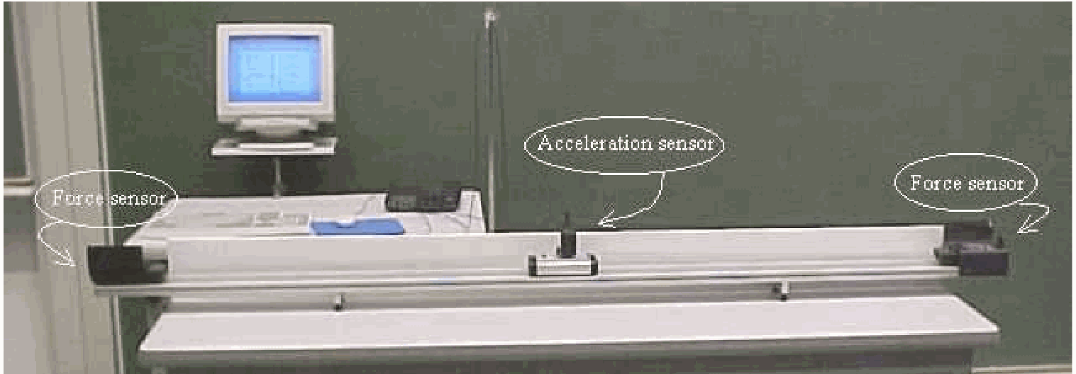
Fig. 325 .#
Equipment#
Lightspot galvanometer
Resistance-box (\(10\mathrm{~k\Omega}\))
Laser
Stopwatch
(Torsionwire model, see Figure 327).
Presentation#
Galvanometer and laser are positioned in such a way that, in the neutral position of the galvanometer, the reflected laser beam is projected on the blackboard behind the laser (see Figure 326). This neutral position is chalk-marked on the blackboard.
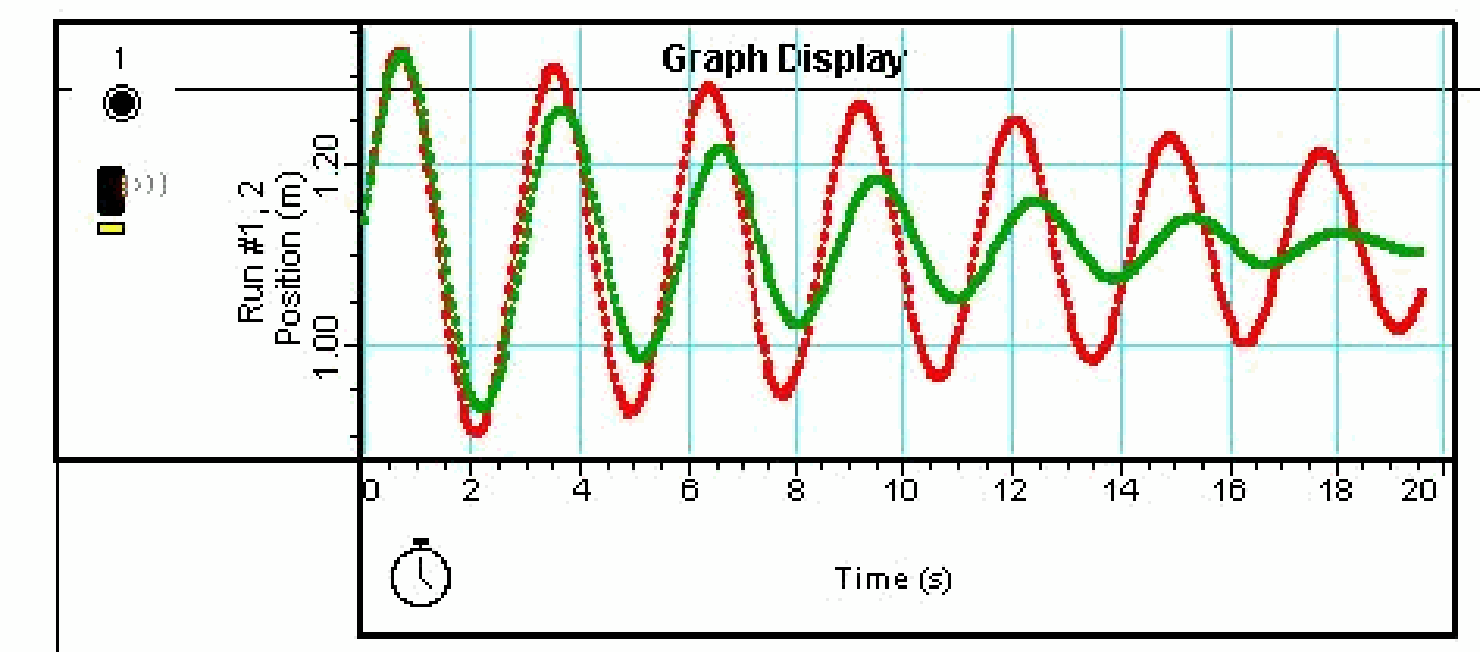
Fig. 326 .#
Now the suspension system of the galvanometer is given a deflection by just touching the leads to the galvanometer with your hands. (Charge on your body usually suffices to make the galvanometer deflect.) The movement of the lightspot on the blackboard shows the free oscillation of the galvanometer-mirror-suspension system. After some oscillations the system comes to rest again. The movement is a damped harmonic motion.
Now the resistance box is connected to the galvanometer (after it has been given a deflection again). The oscillation is observed and the difference in damping, compared to the first situation, is clear. The experiment is repeated with \(10\mathrm{~k\Omega}, 6\mathrm{~k\Omega}\) and \(1\mathrm{~k\Omega}\). We have critical damping using \(6\mathrm{~k\Omega}\) and \(1\mathrm{~k\Omega}\) gives very clear overdamping. Overdamping can be made extreme when the leads are shorted ( \(0 \Omega\) ).
Make the students notice that ‘critical damping’ means ‘reaching equilibrium (the chalk mark) in the shortest time’
When using a stopwatch, it is possible to measure period-times, in order to show the influence of damping on the frequency of the oscillations.
Explanation#
Textbooks give a lot of information about damped harmonic motion. Usually the description is about a simple one dimensional mass-spring system.
The galvanometer-system in our demonstration is a torsion pendulum in which a coil is suspended from a wire. The analysis of such a torsion pendulum can be done analog to that of a mass-spring system.
When the torsion pendulum is twisted an angle \(\theta\) there will be a torque \((\tau)\) that tries to undo the twisting: \(\tau=-\kappa \theta\). ( \(\kappa\) is the torsion constant.) The equation of motion will be:
\(I \ddot{\theta}=-\kappa \theta\) or
\(I \ddot{\theta}+\kappa \theta=0\).
The motion will be a harmonic oscillation with \(\omega^{2}=\kappa / I\) (/ is the rotational inertia). The coil of the galvanometer oscillates in a radial magnetic field and an emf will be induced. The coil is connected to a resistor and a current will flow. A Lorentz force results, giving a torque that counteracts the movement that produces the induction (Lenz’s law) and so this torque will be a damping torque. This damping torque ( \(\tau_{d}\) ) is directly proportional to the angular velocity (like the counter torque in an electric generator): \(\tau_{d}=-r \dot{\theta}\), and now the dynamic equation of motion will be:
\(I \ddot{\theta}+r \dot{\theta}+\kappa \theta=0\) (there is no driving torque).
The demonstration shows a (co)sine-like motion that is multiplied by a factor that decreases in time.
A solution of this differential equation is:
\(\theta=\Theta e^{-\alpha t} \cos \omega t\),
where \(\Theta=\theta\) at \(t=0, \alpha=\frac{r}{2 I}\), and \(\omega^{2}=\frac{\kappa}{I}-\left(\frac{r}{2 I}\right)^{2}\).
\(\alpha=\frac{r}{2 I}\) is a measure of how quickly the oscillations decrease towards zero. The
larger \(r\), the more quickly the oscillations die away. Three cases of damping are distinguished:
Overdamping when \(r^{2}>>4 I \kappa\),
Underdamping when \(r^{2}<4 I \kappa\) and
Critical damping when \(r^{2}=4 I \kappa\). Then equilibrium is reached in the shortest time. \(r\) is changed, when the value of the external resistance is changed, as seen in the Presentation.
\(\omega^{2}=\frac{\kappa}{I}-\left(\frac{r}{2 I}\right)^{2}\) shows that \(\omega\) has a lower value than in the undamped situation. \(\omega\)
Remarks#
When the students have not seen a torsionwire system before, such a system is shortly explained to them using a large scale model (a piece of rope, having a rectangular sheet of metal and a small coil, taped to it. See Figure 327.)
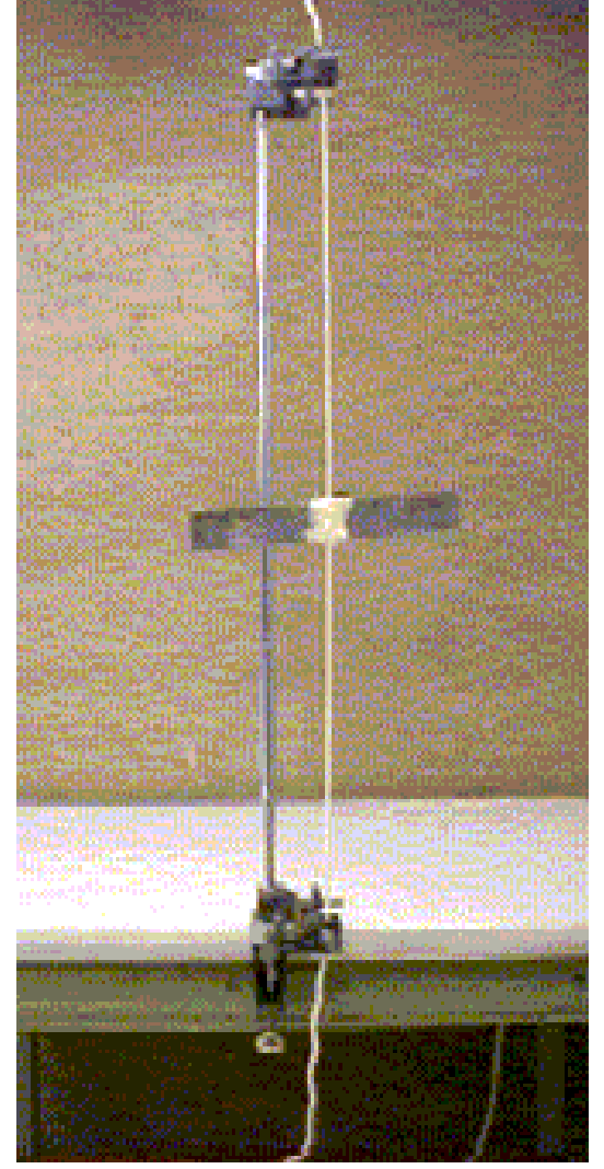
Fig. 327 .#
The resistance-box is placed on a separate table, so that manipulating the box will not disturb the very sensitive galvanometer.
There are three laser spots visible on the blackboard. The first is a reflection of the front glass of the housing of the galvanometer (a fixed spot). The second is the reflection of the mirror (that’s the one we use in the demonstration). The third is a second reflection of the mirror (the first reflection of the mirror reflects partially on the inside of the front glass of the housing) and so shows a double deflection compared to the second spot.
Sources#
Borghouts, A.N., Inleiding in de Mechanica, pag. 264
Mansfield, M and O’Sullivan, C., Understanding physics, pag. 99-101
Roest, R., Inleiding Mechanica, pag. 269
Young, H.D. and Freeman, R.A., University Physics, pag. 411
Alonso, M/Finn, E. J., Fundamentele Natuurkunde, part 1, Mechanica, pag. 278
Giancoli, D.G., Physics for scientists and engineers with modern physics, pag. 374-376