03 LRC Circuits#
Aim#
To show the effect of frequency on current and voltages in an LRC-series (and -parallel) circuit.
Subjects#
5L20 (LCR Circuits - AC)
Diagram#
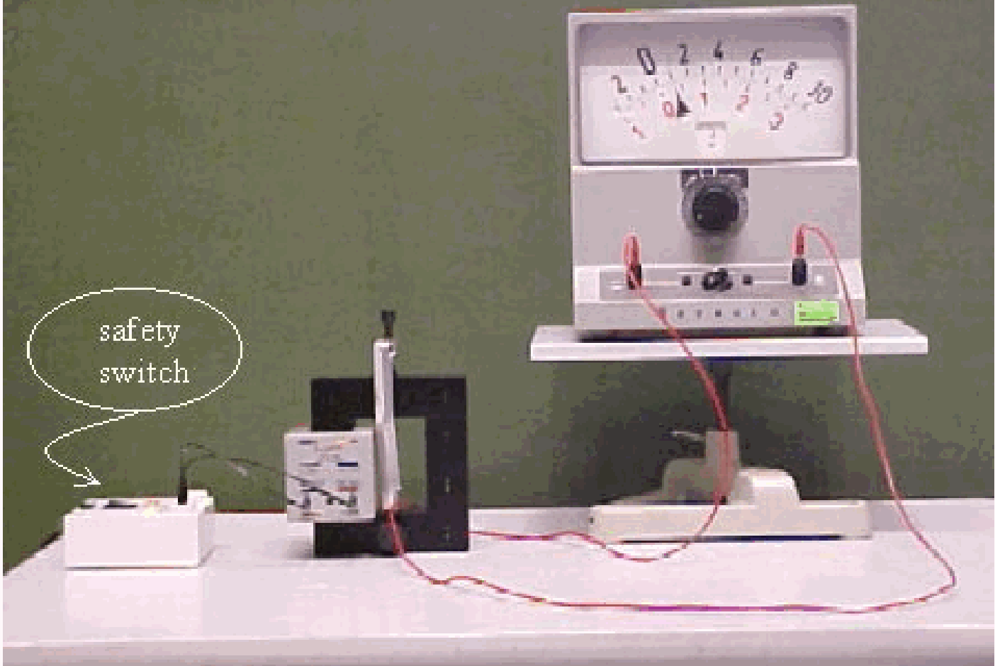
Fig. 555 .#
Equipment#
Signal generator.
Large display to show frequency-setting of signal generator.
Resistance box.
Capacitor box.
Coil, \(n=500\), with iron core.
3 multiscale \(\mathrm{~V}\)-meters.
\(\mathrm{~A}\)-meter.
Presentation#
The circuit is made as shown in Diagram and Figure 556.
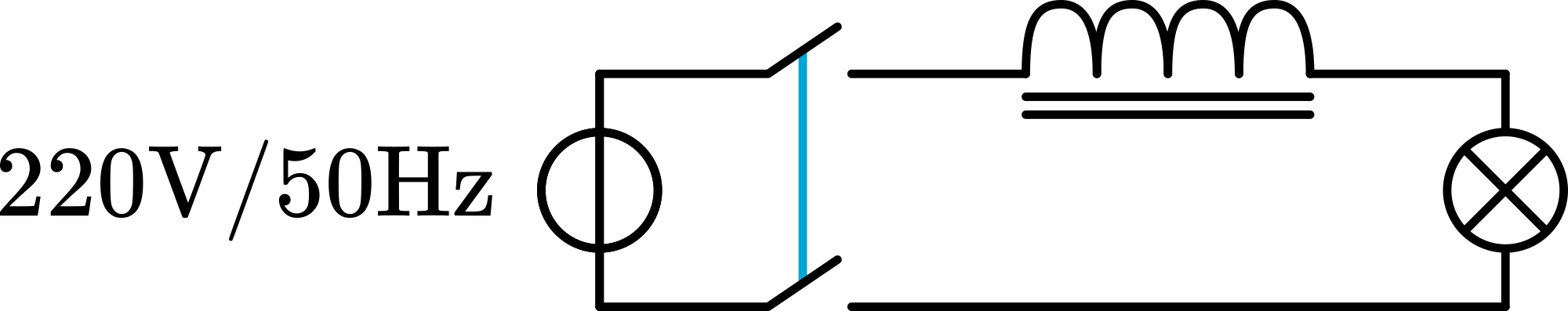
Fig. 556 .#
C is made \(1 u F\). The value of \(R\) is made zero. The voltage of the signal generator is made \(6 \mathrm{~V}\).
The frequency is set at \(100 \mathrm{~Hz}\). Students can read that all the voltage appears at \(\mathrm{C}: \mathrm{V}_{\mathrm{C}}=6 \mathrm{~V} ; \mathrm{V}_{\mathrm{L}}=0 \mathrm{~V}\)
The frequency is made \(10 \mathrm{kHz}\). Students can read that now all the voltage appears at \(\mathrm{L}: \mathrm{V}_{\mathrm{C}}=0 \mathrm{~V} ; \mathrm{V}_{\mathrm{L}}=6 \mathrm{~V}\).
These first two measurements can be discussed now. After this discussion the question is raised: “what happens between \(100 \mathrm{~Hz}\) and \(10 \mathrm{kHz}\) ?”
The frequency is set at \(1 \mathrm{kHz}\). Students can read now that \(\mathrm{V}_{\mathrm{C}}=5 \mathrm{~V} ; \mathrm{V}_{\mathrm{L}}=11 \mathrm{~V}\). When it is the fist time that students are confronted with ac-circuits, these readings will produce many questions: “How is it possible that a \(6 \mathrm{~V}\) power supply gives in the circuit \((11+5=) 16 \mathrm{~V}\) ?; is Kirchhoff’s rule no longer valid?, etc.”. The vectorconcept of ac using a phasordiagram can be introduced to explain the observed phenomenon.
Now it is interesting to explore the region between \(100 \mathrm{~Hz}\) and \(10 \mathrm{kHz}\). Lowering the frequency from \(1 \mathrm{kHz}\) downwards, both \(\mathrm{V}_{\mathrm{C}}\) and \(\mathrm{V}_{\mathrm{L}}\) will rise steeply. We measure at \(670 \mathrm{~Hz} \mathrm{~V}_{\mathrm{C}}=\mathrm{V}_{\mathrm{L}}=140 \mathrm{~V}\) ! Students can also observe that in this situation \(I\) is at a maximum.
The results can be discussed now.
It is easy to change the circuit into a LC-parallelcircuit ( \(R=\infty\) ). \(L\) and \(C\) have now an ammeter in series. Again measurements are made at \(\mathrm{f}=100 \mathrm{~Hz}, \mathrm{f}=10 \mathrm{kHz}\) and \(\mathrm{f}=1 \mathrm{kHz}\) and after that going down to resonance. We measured:
\(-100 \mathrm{~Hz}: I_{\mathrm{C}}=0 ; I_{\mathrm{L}}=.16 \mathrm{~A} ; I_{\text {total }}=.16 \mathrm{~A}\)
\(-10 \mathrm{kHz}: I_{\mathrm{C}}=.35 \mathrm{~A} ; I_{\mathrm{L}}=.0 ; I_{\text {total }}=.35 \mathrm{~A}\)
\(-1 \mathrm{kHz}: I_{\mathrm{C}}=35 \mathrm{~mA} ; I_{\mathrm{L}}=17 \mathrm{~mA} ; I_{\text {total }}=18 \mathrm{~mA}\)
\(-670 \mathrm{~Hz}: I_{\mathrm{C}}=25 \mathrm{~mA} ; I_{\mathrm{L}}=25 \mathrm{~mA} ; I_{\text {total }}=1.4 \mathrm{~mA}\)
These results are similar to those measured in the seriescircuit but now the questions will be raised in relation to the currents.
Explanation#
The first readings of the demonstration can be explained when students have a basic idea of a capacitor and inductance.
Supposing the frequency extremely low (dc) it is clear that a capacitor conducts no current (it is an insulator) and so it will have a very high resistance. At low frequencies the capacitor is charged in a time very small compared to the period time of the ac-source and so the capacitor has constantly the same voltage (almost) as the source. This voltage opposes the source voltage and so no current will flow. At very high frequencies the charging time of the capacitor is equal to or larger than the period time and so the capacitor is charging (and discharging) continuously: a current is flowing.
At extreme low frequencies the coil has a very low inductance (Dt=large) and only a voltage due to its resistance of the copper wires appears across its terminals. At high frequencies the coil will produce a high induced voltage (\(Dt\)=small), so at high frequencies a high voltage can be expected across it. In this qualitative way the opposite frequency-response of C and L can be talked into the students. A more thorough analysis is needed to understand all the results that can be shown in this demonstration. A phase-diagram is needed.
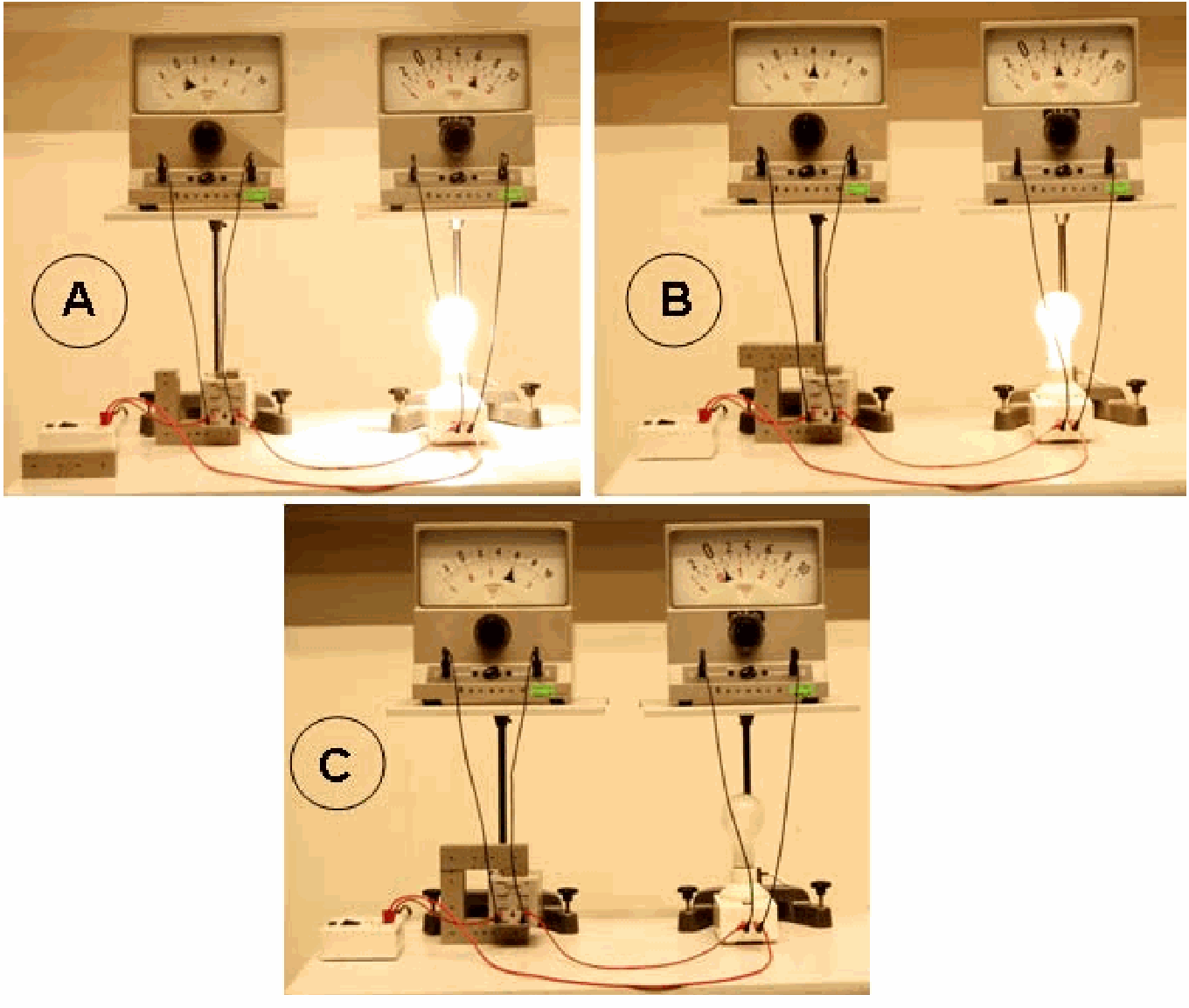
Fig. 557 .#
Many textbooks show these diagrams. Figure 557 shows the diagrams that apply to our demonstrations.
The explanation of the results measured in the parallel circuit can be explained using a current phase-diagram.
Remarks#
A lot more can be shown with this demonstration. For instance the influence of \(R\).
Also a mathematical analysis is possible using the capacitance \(X_{C}=(\omega C)^{-1}\) and inductance \(X_{\mathrm{L}}=\omega \mathrm{L}\). Many textbooks show how to do this.
Sources#
Mansfield, M and O’Sullivan, C., Understanding physics, pag. 531-535
McComb,W.D., Dynamics and Relativity, pag. 84-86
Roest, R., Inleiding Mechanica, pag. 281-283
Young, H.D. and Freeman, R.A., University Physics, pag. 987-1013