5H40.03 Lorentz Force (2)#
Aim#
To show the force on a current carrying wire in a magnetic field.
Subjects#
5H40 (Force on Current Wires)
Diagram#
Fig. 510 .#
Equipment#
Conducting wire \((\mathrm{I}=2 \mathrm{~m})\).
A-meter ( \(0-1 \mathrm{~A}\) ).
Current source ( \(0-1 \mathrm{~A}\) ).
Strong horseshoe magnet (we use \(\mathrm{B}=0.5 \mathrm{~T}\) ).
Overhead projector
Presentation#
The wire is loosely hung over the overhead projector, so it can swing (see Diagram A). The picture of the wire is sharply projected on the blackboard (see Diagram B).
By hand, the wire is given a deflection in order to show that for such a deflection only a small force is needed. The larger the deflection, the larger the force. (For small deflections, the deflection is proportional to the force.) Now the horseshoe magnet is placed on the overhead projector. The wire is in the middle of the gap between the North- and the South pole. Mark this position of the wire on the blackboard. Slowly raise the current and observe that the wire deflects. The relationship between the direction of current, direction of magnetic field and direction of force is observed. Reverse the current and see that the force is directed towards the other side now. Also the horseshoe magnet can be turned.
Raising the current in steps and marking the position of the wire on the blackboard, it can be observed (roughly) that the Lorentz force is proportional to the current.
Explanation#
Applying Biot-Savart’s law it can be shown that the force on a current element \(\Delta \vec{l}\) in a magnetic field of flux density \(\vec{B}\) is given by \(\vec{F}=I \Delta \vec{l} \times \vec{B}\). In our case, having \(\vec{B}\) perpendicular to \(\Delta \vec{l}\) and considering that the wire-element in the field is straight, then \(F=I I B\). Our demonstration verifies \(F \propto I\).
Remarks#
Verifying \(F \propto I\) supposes that only the displacement of the wire between the magnetic poles is considered. Only in this region the magnetic field is uniform and \(\vec{B}\) can be considered constant.
The demonstration can also be used to estimate the value of the fluxdensity B. In \(F=I / B_{f}\) \(I\) and /are known (see Figure 511).
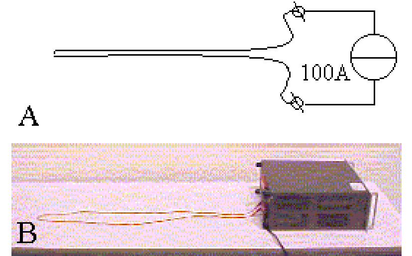
Fig. 511 .#
\(I\) is given such a value that it deflects the full width of the gap between the poles \((2 \mathrm{~cm})\). (In our case the current needed for that is .5A.) The force needed for such a deflection can be estimated when we know the mass of the suspended wire. (In our case: \(\mathrm{m}=.032 \mathrm{~kg}\), so \(\mathrm{F}=(1 / 40) \cdot(.032) \cdot(10)=8 \mathrm{mN}\). Then \(B\) will be \(.3(2) \mathrm{T})\).
Video Rhett Allain#
Sources#
Mansfield, M and O’Sullivan, C., Understanding physics, pag. 486-487
Young, H.D. and Freeman, R.A., University Physics, pag. 880-881