01 Balmer Series#
Aim#
To show the visible hydrogen spectrum and its regularity.
Subjects#
7B10 (Spectra)
Diagram#

Fig. 658 .#
Equipment#
Gas discharge lamp, filled with water vapor.
High voltage power supply, 3.5kV \(V_{r m s}\). (see Safety)
Lens, \(\mathrm{f}=+50 \mathrm{~mm}\) (used as condenser lens).
Lens, \(+150 \mathrm{~mm}\) (to focus the slit on the camera-screen).
Adjustable slit.
Grating \(100 \mathrm{~lines/mm}\).
Camera, lens removed.
Linear positioner.
Optical rail.
Beamer.
Large sheet of black paper, rolled as a tube (see Diagram B).
Safety#
The high voltage power supply is operated from the AC mains outlet. Always disconnect the mains plug from the wall outlet before making any changes to the demonstration setup (e.g. changing the Balmer lamp or changing the fuse). See the Leybold Didactic instruction sheet.
Presentation#
Preparation#
The gas discharge lamp and the two lenses are placed on the optical rail. The power supply of the lamp is switched on. Steady discharge is reached after approx. 15 minutes (see “notes on operation” of Leybold Didactic).
The \(+50 \mathrm{~mm}\) lens is shifted close to the lamp to focus as much light as possible through the \(+150 \mathrm{~mm}\) lens. Both lenses are fixed. Then the variable slit and camera (mounted on the linear positioner and connected to the beamer; see Figure 659) are positioned on the optical rail. The slit is shifted to image it sharply on the camera CCD-screen. The linear positioner is shifted also, until the slit can be seen on the middle of the projected image.
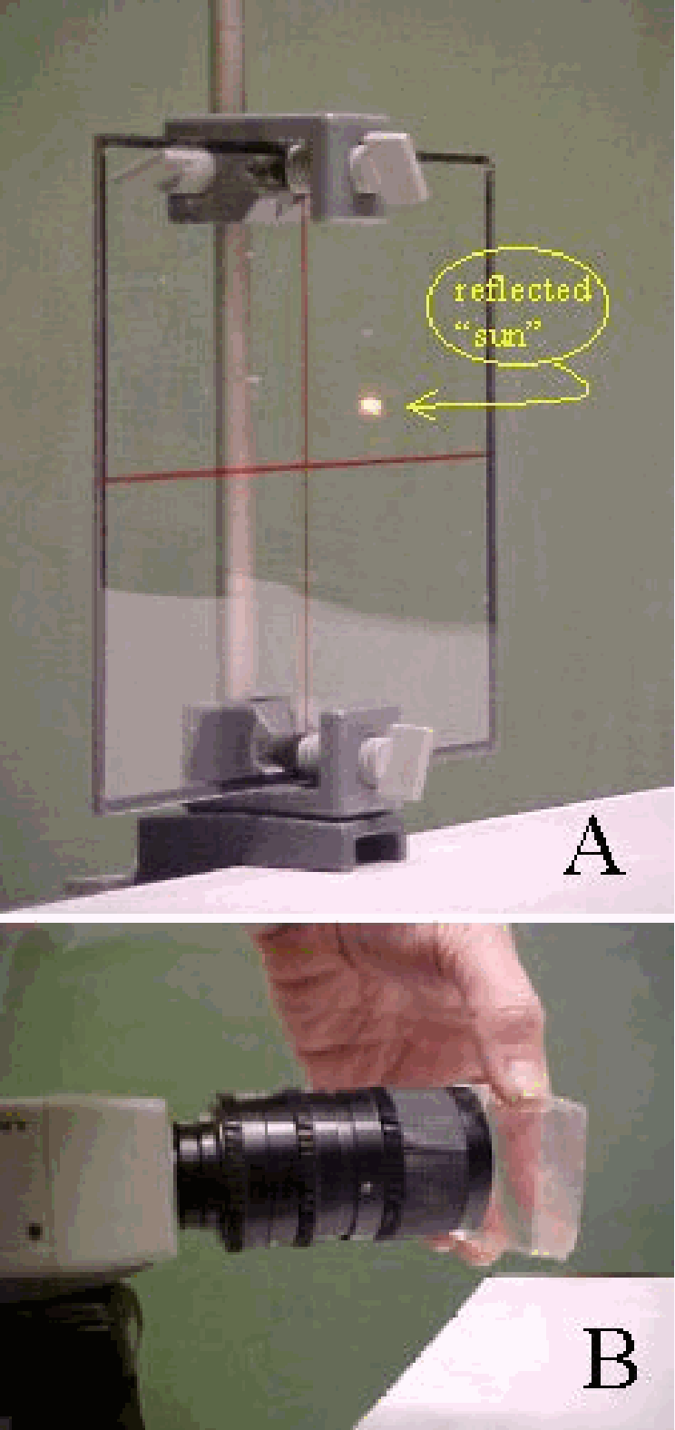
Fig. 659 .#
Demonstration#
The room is darkened and a sharp and intense image of the slit is visible to the audience. Then the grating is placed in its holder as close as possible to the camera. We also place the black tube around the set-up (see Diagram B). Blue and red lines appear (also a fainting of the slit-image can be observed when the grating is placed). In this way we have build a spectroscope, like Fraunhofer did (1814).
The students are invited to describe what they see:
Fig. 660 .#
“… diffraction pattern of a grating; first and second orders on both sides of the central maximum; blue is closer to the central maximum then red; …”
We shift the camera sideways so that the central maximum is on one side of the projected image. Then we ask the students what will happen when we shift the grating away from the camera. After their answering we shift it away and observe the broadening of the orders, but the pattern remains the same. In the shifting also a faint violet line ( \(v\) ) can be seen.
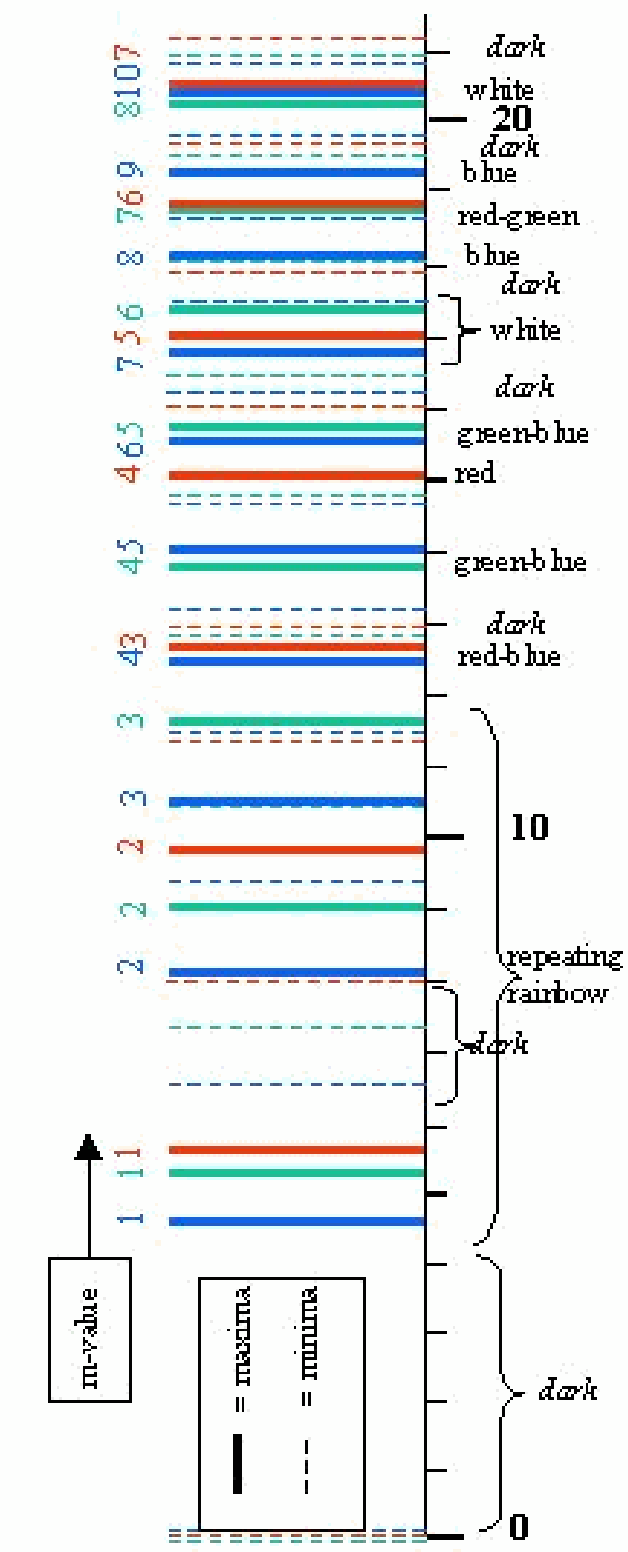
Fig. 661 .#
The image is partly projected on the blackboard and we indicate with chalk the horizontal positions of: Central maximum (Cm), violet(v) -, blue(b) - and red(r) line. With a measuring tape we found:
\(Cm-v=170 \mathrm{~cm}\)
\(Cm-b=188 \mathrm{~cm}\)
\(Cm-r=256 \mathrm{~cm}\)
An explanation of what is observed now follows.
Explanation#
Calibration is performed by using \(\sin \theta=\frac{\lambda}{d}\) (first order maximum of a diffraction pattern created by a grating, \(d\) being the distance between the slits of the grating.), see Figure 660.
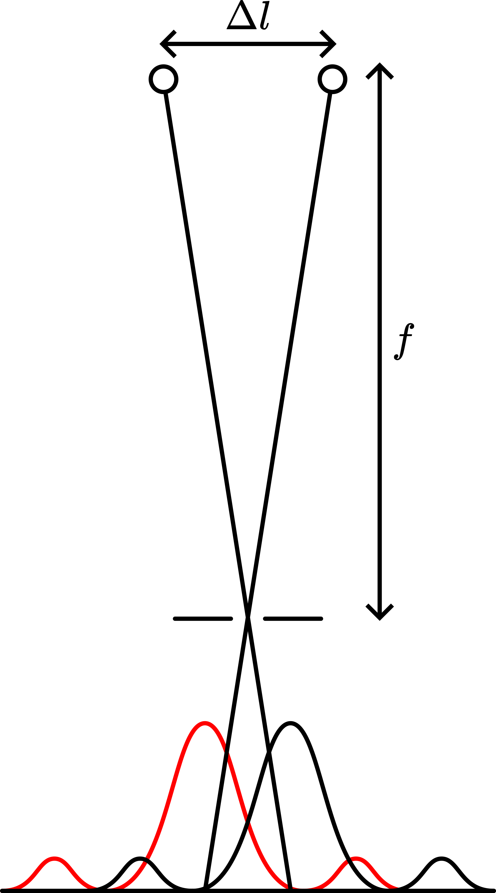
Fig. 662 .#
Figure 660 shows: \(\sin \theta=\frac{x}{\sqrt{x^{2}+s^{2}}}\). Rewriting we get: \(x=s \frac{\lambda}{\sqrt{d^{2}-\lambda^{2}}}\). When \(\lambda \ll d\) then \(x\) is directly proportional to \(\lambda\). Since we do not know s exactly we cannot calibrate our spectroscope. But we can compare the different first order colors like Balmer did. Using our tape measurements we find:
The empirical formula as stated in 1885 by Balmer (while studying the experimental results of Ångström) says: \(\lambda_{5}, n=3,4, \ldots\)
Using the right numbers for \(n\) gives us:
Now calculating: \(\frac{\lambda_{4}}{\lambda_{3}}=1,35 ; \frac{\lambda_{5}}{\lambda_{3}}=1,51 ; \frac{\lambda_{5}}{\lambda_{4}}=1,12\).
The conformity with the results obtained in our simple demonstration is striking, and we identify \(\lambda_{3}\) as the red line, \(\lambda_{4}\) as the blue line and \(\lambda_{5}\) as the violet line.
The measurements are easy; the excellence of Balmer is in the mathematical formulation. He really did a terrific job
Sources#
Giancoli, D.G., Physics for scientists and engineers with modern physics, Third edition, pag. 900-901 and 963-965.
Wolfson, R., Essential University Physics, First edition, pag. 616.