01 Hooke’s Law#
Aim#
This demonstration shows Hooke’s law. However, the focus is on taking measurements, measurement uncertainty and how to interpret the results.
Subjects#
1A20 (Error and Accuracy)
1R10 (Hooke’s Law)
Diagram#
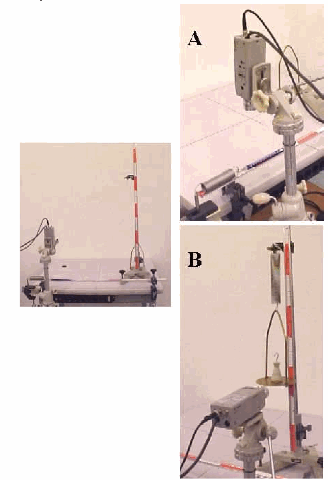
Fig. 4 .#
Equipment#
Spring \((k=50 \text{ N} / \text{m})\) with pre-stress \((2.5 \text{N})\).
Two rulers.
Spring balance, 10N.
Scale to be attached to spring balance (heavier than \(250 \mathrm{g}\)).
Mass: 200.0g.
Video-camera.
Beamer to project camera image.
Presentation#
One ruler is placed horizontal. The spring is fixed to the ruler and can slide along when it is pulled by the spring balance (see Diagram A). The camera is positioned in such way that the position of the spring on the ruler and the force indicated by the spring balance are recorded: all students ought to be able to read the results.
The second ruler stands vertical. The spring, with the scale fixed to it, hangs close to the ruler (see Diagram B). The camera records the position of the spring on the ruler.
We start with the horizontal arrangement. First, the equilibrium position ( \(F=0 \text{ N}\) ) is read. Then the spring is given a displacement \((x)\) of \(5.0 \text{ cm}\) from its equilibrium. The corresponding force is read and the spring constant \((k)\) is calculated: \(k=\frac{F}{x}\). In our case, we find: \(x=5.0 \text{ cm} ; F=5.7 \text{ N}\); so \(k=114 \text{ N/m}\). Its associated uncertainty (\(u\)) is calculated:
We find: \(u(x)=0.1 \text{ cm} ; u(F)=.1 \text{ N}\); so \(u(k)=3 \text{ N/m}\).
The spring and scale are now fixed next to the vertical ruler. The camera is turned horizontally and records the position of the spring. First, the equilibrium position \(\left(h_{0}\right)\) is read. Then the mass of \(200.0 \text{~g}\) is placed on the scale. The displacement of the spring \(\left(h_m\right)\) is read and the spring constant \((k)\) is calculated: \(k=\frac{m g}{\left|h_{m}-h_{o}\right|}\). We find: \(h_{0}=35.6 \text{ cm} ; h_{m}=38.8 \text{ cm}\); using \(g=9.812\); so \(k=61.3 \text{ N/m}\). Also the uncertainty (\(u\)) is calculated:
in which \(u(v)\) is determined by \(v=\left|h_{o}-h_{m}\right|\) and \(u(v)^{2}=u\left(h_{o}\right)^{2}+u\left(h_{m}\right)^{2}\). We find: \(u(\mathrm{~m})=0.1 \text{~g}\); \(u\left(h_{o}\right)=u\left(h_{m}\right)=0.1 \text{ cm} ; u(g)=0.001 \text{~m} / \text{s}^{2}\); so \(u(k)=3 \text{ N} / \text{m}\). Terms with \(m\) and \(g\) are negligible in \(u(k)\).
The two results are not in good agreement: the difference between the two calculated \(k\)-values is larger than two times the uncertainty (\(|k_1-k_2|>2\sqrt{u_{k_1}^2+u_{k_2}^2}\)). The students are asked to discuss the possible cause of these conflicting results. After some time the word “pre-stress” appears in the student group.
Explanation#
The spring is pre-stressed \(\left(F_p\right)\), so \(k=\frac{F-F_{p}}{x} \cdot k\) is not proportional with \(F\), there is only linearity between \(k\) and \(F\). More measurements (\(F=F(x)\)) and making a graph will produce significant values.
In our case we find \(F_p=2.66 \text{ N}\) with \(u(F)=0.08 \text{ N}\) and \(k=56.7 \text{ N/m}\) with \(u(k)=1.3 \text{ N/m}\).
Remarks#
This demonstration is shown in our Introductory Laboratory Course.
The first reading of \(x=5.0 \text{cm}\) also has two error margins, so \(u(x)\) is actually higher (\(u(x)^{2}=0.02\)), and \(\left(u(k)=5 \text{ N/m}\right)\).