05 Simple Harmonic Motion (SHM) (3)#
Aim#
To show simple harmonic motion of a spring-mass system and the relationship between the variables that determine the period.
Subjects#
3A40 (Simple Harmonic Motions)
Diagram#
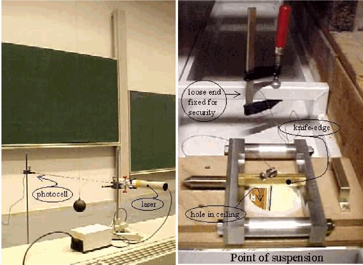
Fig. 319 .#
Equipment#
Two identical helical springs (we use \(\mathrm{k}=45 \mathrm{~N} / \mathrm{m}\) ).
Two masses of \(1 \mathrm{~kg}\).
Demonstration ruler with sliding markers.
Large stopwatch.
Position sensor.
Interface and software.
Projector to project monitor screen.
Clamping material.
Presentation#
One spring is hung to a hook and loaded with \(1 \mathrm{~kg}\). The extension is observed and the spring constant \(k\) can be determined.
The software is set up to display a graph of position-time. By hand the mass is displaced more vertically and released. Now the mass oscillates: a linear translational motion confined to the vertical direction. After some time data collection is started. We collect data during around 10 seconds. It can be observed that the position-time graph has a sinusoidal shape. To verify this, we select a little more than one cycle displayed on the screen and then have the software make a sine-fit. A black-lined sine is drawn in the red-colored collected data and the fit is unmistakable correct (within certain limits, see Figure 320: \(\mathrm{CHI}^{2}=0.002254\), the smaller this number, the better the agreement between collected data and the mathematical sine).
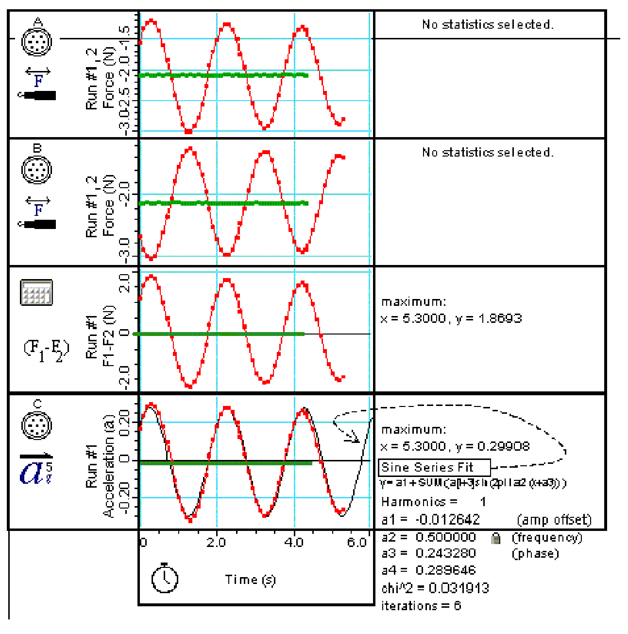
Fig. 320 .#
The mass is set in oscillatory motion again. The stopwatch is started and the time needed for ten oscillations is measured. \(\omega=\sqrt{\frac{k}{m}}\) can be verified.
The mass hung to the spring is doubled. Let students predict what will happen to the period. Set the system in motion and again clock ten periods to check if the prediction fits.
Two springs are connected in series. This combination is loaded with 1 \(\mathrm{kg}\) and the spring constant of this combination can be determined. Also this series combination can be loaded with one or two kg and set in oscillatory motion and wchecked.
The same can also be performed when the two identical springs are positioned parallel.
Explanation#
A simple mass-spring system oscillates with a frequency \(\omega=\sqrt{\frac{k}{m}}\). So doubling the mass will lower the frequency by a factor \(\frac{1}{\sqrt{2}}\).
When two springs are connected in series, this combined spring will have a “new” spring constant of \(k_{3}=\frac{F}{x_{1}+x_{2}}\) (see Figure 321). F acts everywhere in the combined system, so \(x_{1}=F / k_{1}\) and \(x_{2}=F / k_{2}\). This yields \(k_{3}=\frac{k_{1} k_{2}}{k_{1}+k_{2}}\).
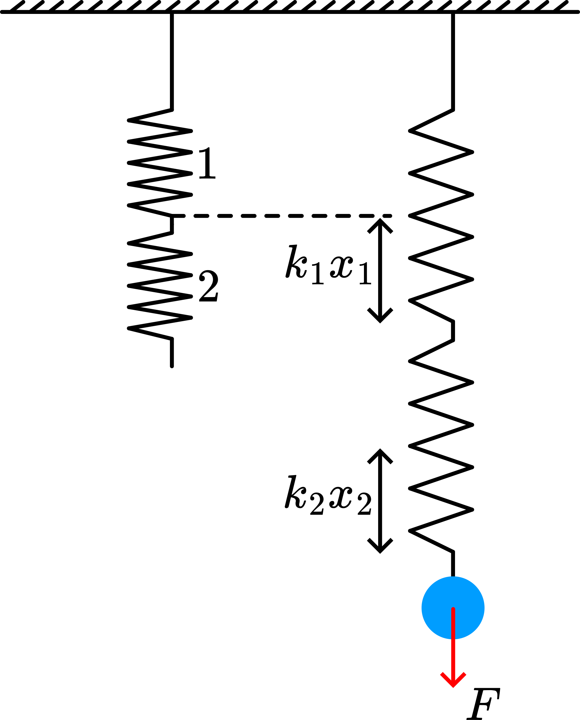
Fig. 321 .#
In our demonstration \(k_{1}=k_{2}(=k)\), so \(k_{3}=1 / 2 k\). The frequency will change according to \(\omega=\sqrt{\frac{k}{m}}\). So a system with two springs in series and two masses added to it will have half the frequency of one mass suspended to one spring.
When two springs are connected parallel: \(k_{1} x_{1}+k_{2} x_{2}=F=k_{3} x\). \(k_{3}=F / x\) (see Figure 322), so \(k_{3}=\frac{k_{1} x_{1}+k_{2} x_{2}}{x}\).
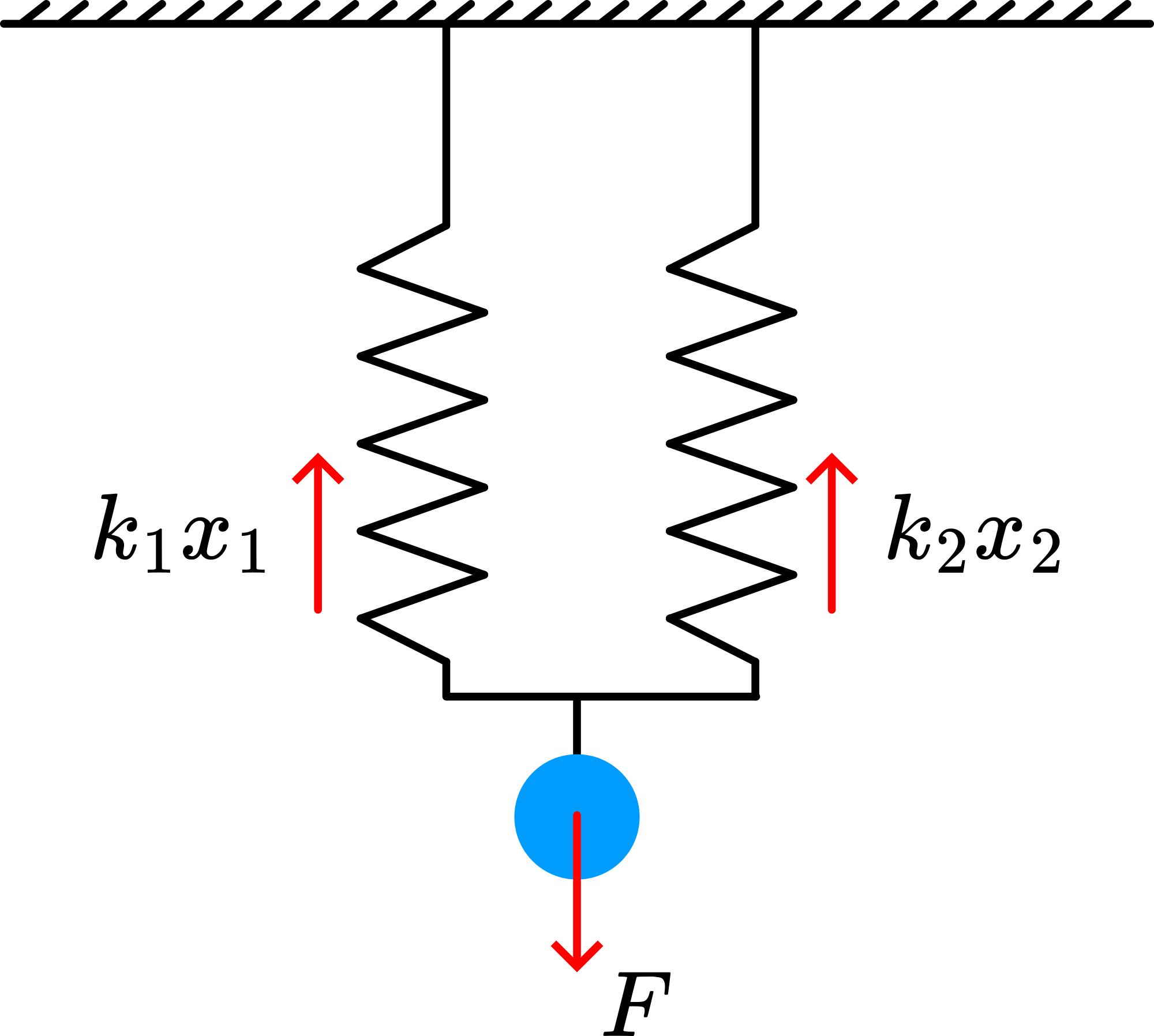
Fig. 322 .#
When the system is made in such a way that \(x_{1}=x_{2}\), then \(x_{1}=x_{2}=x\) and \(k_{3}=k_{1}+k_{2}\). So in our demonstration \(k_{3}=2 k\). So a system with two springs in parallel and two masses added to it will oscillate with the same frequency as when one mass is suspended to one spring. The measured \(\omega\) s can be verified now.
Sources#
Mansfield, M and O’Sullivan, C., Understanding physics, pag. 48-52, 89 and 97-101
McComb,W.D., Dynamics and Relativity, pag. 81-82