05 Plucking a String#
Aim#
To show the frequency-components in a plucked string and how they depend on the strings tension.
Subjects#
3B22 (Standing Waves)
3C50 (Wave Analysis and Synthesis)
Diagram#
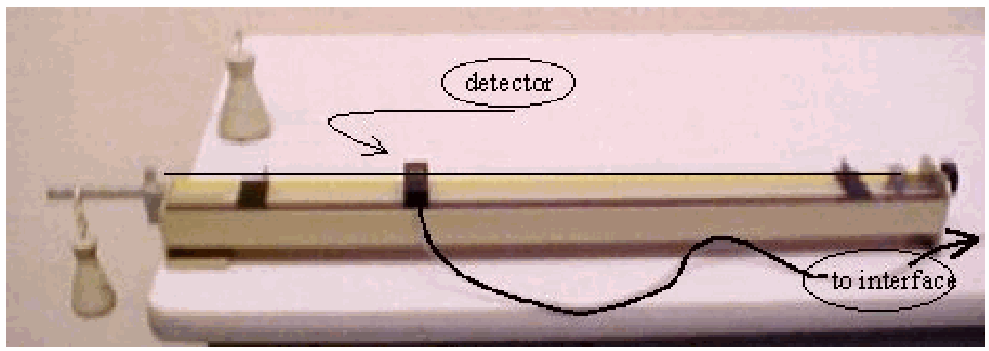
Fig. 365 .#
Equipment#
Sonometer with detector.
Steel string, \(\varnothing=0.5 \mathrm{~mm}\left(\mu=1.5 \times 10^{-3} \mathrm{~kg} / \mathrm{m}\right)\).
Two masses ( \(0.5 \mathrm{~kg}\) and \(1 \mathrm{~kg}\) ).
Data-acquisition system.
Presentation#
Set up the demonstration as shown in Diagram and connect the detector, that is placed near the string, to the interface. The software is set up to have an oscilloscope screen and an FFT display (frequency spectrum) as in Figure 366.
Load the string with . \(5 \mathrm{~kg}\) (see Diagram, mass hanging at the end of the lever). Pluck, by hand/nail, the string (moving it in a vertical direction). We do this in two ways:
a. Pluck the string in its centre.
The scope display shows a more or less symmetric shape. The FFT display shows the frequency components in it. Using the crosshair cursor we read: \(102-, 289-, 473-, 663 \mathrm{~Hz}\). Very roughly the relationship \(1:3:5:7\) is visible in these frequencies.
b. Pluck the string close to its end.
The scope display shows a more or less sawtooth shape, and while it dampens becomes more or less sinusoidal. The FFT display shows the frequency components in it. The fundamental frequency is very high compared to the higher harmonics. (Using the crosshair cursor we read: \(102-, 190-, 288-, 385-, 473-, 570-, 666-, 755-, 853\mathrm{~Hz}\), etc. Very roughly the relationship \(1: 2: 3: 4: 5: 6: 7: 8: 9\) is visible in these frequencies.)
Loading the string with another force.
a. By hand.
When the string is plucked, we pull the weight. We see on the FFT-display shift the frequency components to higher frequencies.
b. Load the string with \(1 \mathrm{~kg}\).
Again the string is plucked, first in its centre, and next close to its end. The observed frequencies are now:
2a: \(140-, 268-, 405-, 541-, 677-, 799-, 939\mathrm{~Hz}\);
2b: \(140-, 405-, 678\mathrm{~Hz}\) (see Figure 366).
Compare these data with the results of the first part of our demonstration and show that the ratio’s \(140 / 102 ; 268 / 190 ; 405 / 288 ; 541 / 385\); etc. are all very close to \(\sqrt{2}\).
Fig. 366 .#
Simulation:#
To support the results of our demonstration we show the simulation of a vibrating string. To do so we choose “Loaded String Simulation”, a JAVA-Applet on the site https://www.falstad.com/ in which the string can be plucked at different points using the mouse. Adjusting the simulation speed top ‘low’ the vibrating string is shown in slow motion, clearly showing its frequency amplitude components (and its first three phasors). You can hear also the sound of the plucked string and observe the difference between a centre-pluck and an end-pluck.
Explanation#
Grasping a string near its end to pluck it, makes the triangular shape in the oscillating string to be expected. The FFTdisplay distincts a fundamental frequency and a number of its harmonics. In general a triangular shape appears when to a fundamental frequency a second harmonic (first overtone), a third harmonic (second overtone), etc. is added. The demonstration verifies this.
Grasping the string in its centre to make it oscillating, a symmetric waveform is to be expected with uneven harmonics in it.
When the crosshair cursor is used in the FFT-display to read the observed frequencies it shows that doubling the string’s tension means a factor \(\sqrt{2}\) in increase in frequency.
A standing wave occurs when traveling waves/pulses after their reflections at the end of the string interfere positively, giving large standing amplitudes. The speed of pulses/waves traveling along the string is: \(v=\sqrt{\frac{F}{\mu}}\), (see Speed of a single pulse on different strings (1). \(v=f \lambda\) and so: \(f=\frac{v}{\lambda}=\frac{1}{2 L} \sqrt{\frac{F}{\mu}}, \angle\) being the length of the string. Our demonstration in doubling the string tension \((F)\) verifies the square root of \(F\) in relation to \(f\).
(When we fill up the formula \(f=\frac{v}{\lambda}=\frac{1}{2 L} \sqrt{\frac{F}{\mu}}\) with the data of our demonstration we calculate a fundamental frequency of \(115 \mathrm{~Hz}\) (Demonstration yields \(102 \mathrm{~Hz}\) ).
That many frequencies occur in a plucked string can be explained by showing the solution on the one-dimensional wave equation. This equation, \(\frac{\partial^{2} f}{\partial x^{2}}-\frac{1}{c^{2}} \frac{\partial^{2} f}{\partial t^{2}}=0\),
can generally be solved by: \(f(x, t)=f_{1}\left(t-\frac{x}{c}\right)+f_{2}\left(t+\frac{x}{c}\right)\) (d’Alembert solution), where \(f_{1}\) and \(f_{2}\) can be any function. So \(f_{n}\) can be any time-harmonic solution like \(A e^{-i \omega(t-x / c)}+B e^{-i \omega(t+x / c)}+C e^{i \omega(t-x / c)}+D e^{i \omega(t+x / c)}\), etc., in which \(\omega\) can have many values.
For a string with fixed ends we get a number ( \(n\) ) of possible standing waves; \(n\) different modes of vibration: \(\omega_{n}=n \omega_{1}, n=1,2,3, \ldots \omega_{1}\) is called fundamental frequency, the others harmonics or overtones.
Sources#
Mansfield, M and O’Sullivan, C., Understanding physics, pag. 344-345 and 349-350
Young, H.D. and Freeman, R.A., University Physics, pag. 627-630