01 Gauss’ Law#
Aim#
In order to introduce Gauss’s law, the analogy between the velocity field of a fluid flow and the electric field is used.
Subjects#
5B20 (Gauss’ Law)
Diagram#
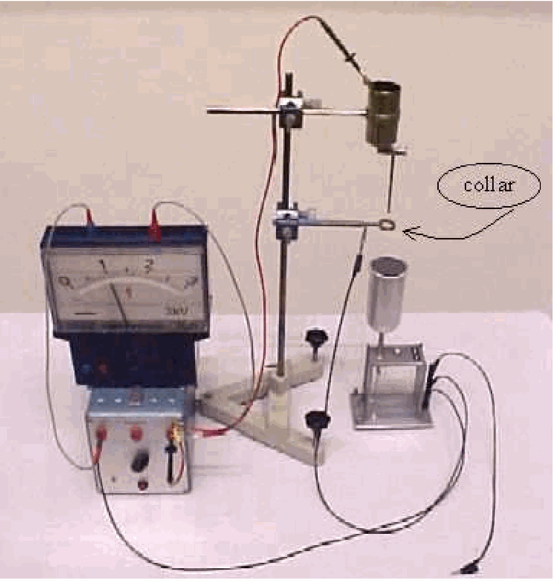
Fig. 460 .#
Equipment#
Two circular clear acrylic plates, separated by \(0.5 \mathrm{~mm}\)
Glass tray in which the assembly of circular plates fits easily (see Diagram).
Syringe \((2 \mathrm{~mL})\), with small needle and filled with ink.
Separating funnel \((1 \mathrm{~L})\).
Overhead projector.
Presentation#
The assembly of the clear acrylic plates is placed in the glass tray and positioned on the overhead projector. A flexible tubing of around \(50 \mathrm{~cm}\) is connected to the central connector in the upper circular plate. The glass tray is filled with water until the assembly of circular plates is submerged. Using Hoffman clamps, the flexible tubing is filled with water. The needle of the syringe is stuck into the flexible tubing just above the connection to the plates (see DiagramB).
Slowly the Hoffman clamp is opened just a little so that a slow fluid flow occurs between the plates. The 1 liter-separating funnel is made dripping in order to keep the level in the flexible tubing constant and, in that way, the flow constant. Then the ink marker is injected into the fluid stream and the spreading of the fluid between the circular plates can be observed.
Placing radial distance marks on the circular acrylic plates, the velocity of the fluid can be determined directly by measuring the crossing times of the leading surface of the ink marker. The feature of the decrease in velocity as a function of radial distance is strikingly obvious and in agreement with \(1 / r\) dependence.
When this result is solidified, the demonstration is followed by a theoretical exercise of applying the same analysis to a fluid source that is allowed to expand outward uniformly in three dimensions. This will lead to a \(1 /r^{2}\) dependence (see Explanation).
Once the analogy between \(E=Q / 4 \pi \varepsilon_{0} t^{2}\) and \(v=f / 4 \pi t^{2}\) is established, students are asked to identify the electric quantities that are analogues to the velocity, \(v\), and the fluid flow \(f\). These quantities are the electric field \(E\), and \(Q / \varepsilon_{0}\), respectively. Since both electric field and velocity are linear quantities an equivalent of the continuity principle \(f=v A\) must also exist for electric fields. Given the analogies, students will find this electric continuity principle as \(Q / \varepsilon_{0}=E A\) : Gauss’s law! (The term \(E A\) has then rightfully the meaning of “electric flux”)
Explanation#
The continuity-relation between the volume rate of flow, \(f(f=\Delta V / \Delta t)\), the fluid velocity, \(v\), and the cross-sectional area, \(A\), is \(f=v A=\) constant. Challenging the students to consider the flow in this system they find, once the area \(A\) is identified as \(2 \pi r d\) (and so \(2 \pi r d v=\) constant), the \(1 / r\) dependence of the velocity field in this essentially two-dimensional system.
In case of three-dimensional flow the area \(A\) considered equals \(4 \pi r^{2}\) giving \(4 \pi r^{2} v=\) constant leading to the \(1 / r^{2}\) dependence.
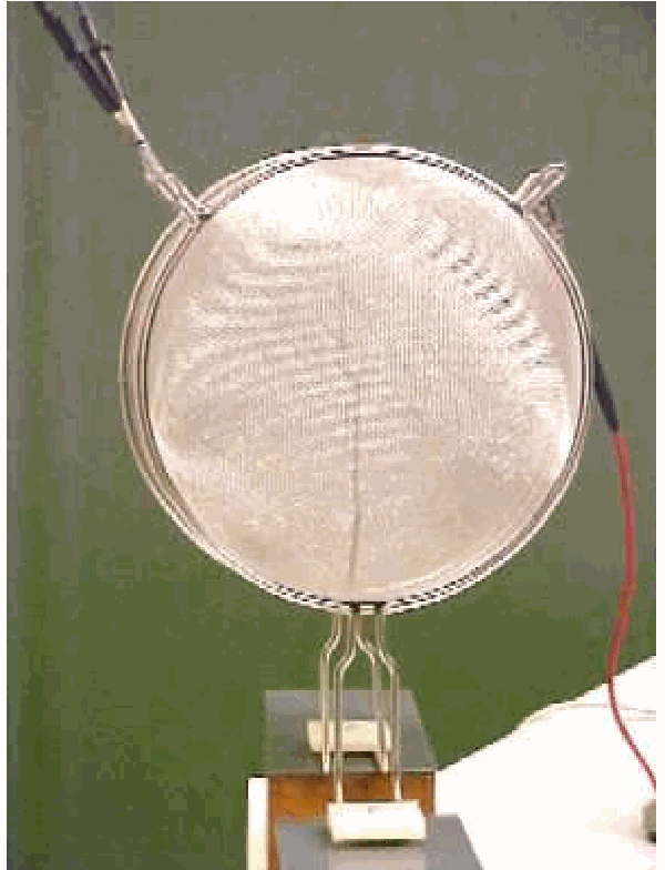
Fig. 461 .#
Remarks#
Comparing electric flux and fluid flux offers insight, but do not get them confused: An electric flux is not a flow of any substance! Flux can be defined for any vector field.
The support for the separating funnel is not fixed to the overhead projector but to a separate table (see Diagram). This is done on purpose, because otherwise adjusting the dripping of the funnel makes the assembly shaking and that will disturb the observed fluid flow.
Instead of an overhead projector also a camera can be used to show the fluid flow.
Filling the flexible tubing of \(50 \mathrm{~cm}\) is done by using two Hoffman clamps (see Figure 462).
Take care that no air bubbles are in the fluid between the two circular plates. (We use a piece of overhead-sheet to wipe away bubbles.)
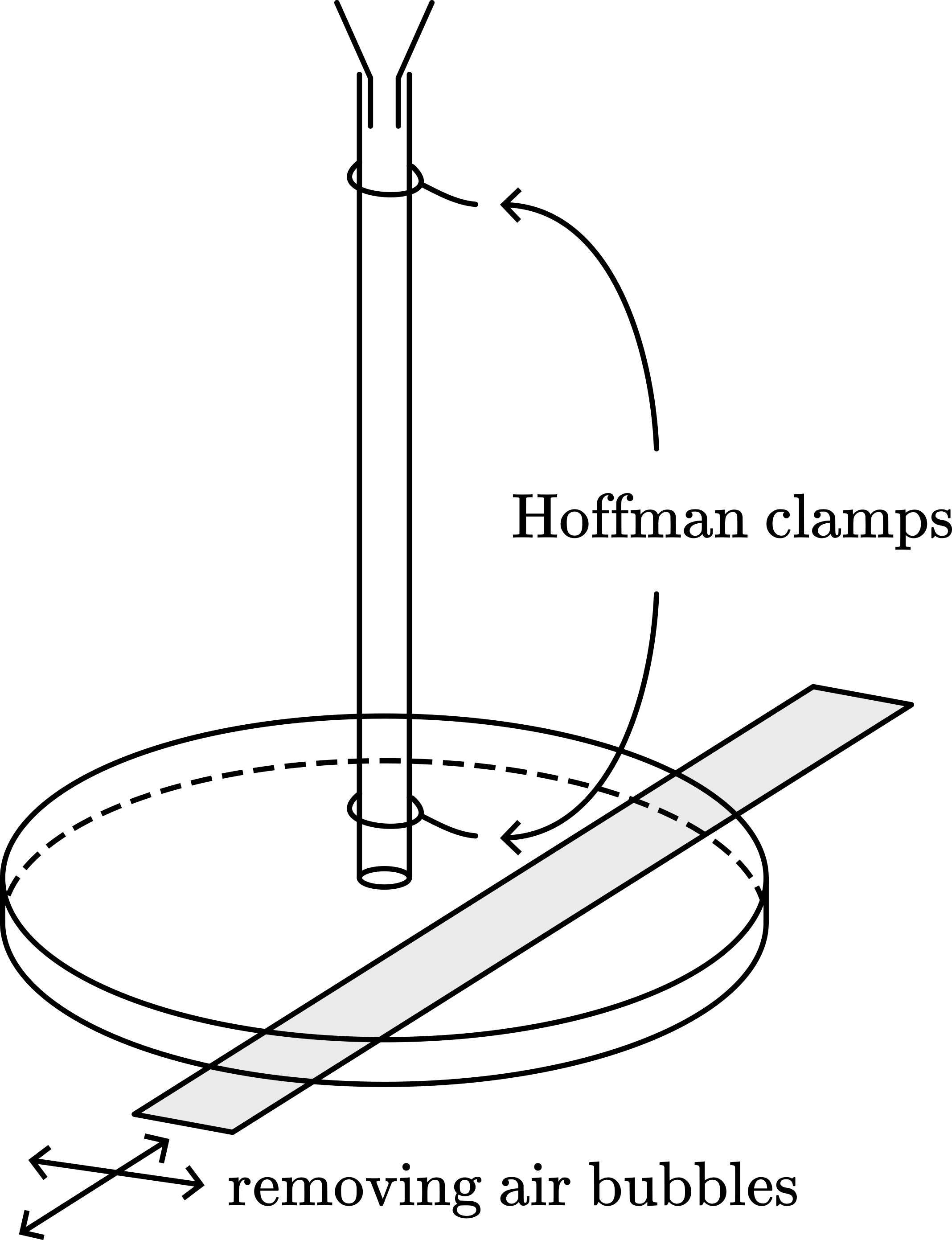
Fig. 462 .#
Sources#
Giancoli, D.G., Physics for scientists and engineers with modern physics, pag. 578 (upper part)
American Journal of Physics, pag. Vol. 72, 1272-1275